MiniGPT (Part 1)
Neil Haddley • October 5, 2026
How a GPT runs: a real trained MiniGPT taken apart while it writes, explained with pictures and a wheel of chances, then traced line by line through Jibin Joseph's notebook code, with the trained model to download and run yourself
Nobody programs a large language model (LLM)'s knowledge in directly: it is grown, by training. I spend a lot more of my time using LLMs to write code, emails, blog posts etc. than I do thinking about how they are built but it seems reasonable that understanding how LLMs are made will help me to apply them better. In any case, I am naturally curious, and I want to be able to explain how they work.
I started this effort in July 2023 with the book Generative AI with Python and TensorFlow 2, by Joseph Babcock and Raghav Bali. More recently, I found the paper MiniGPT: Rebuilding GPT from First Principles by Jibin Joseph, and decided to use it for some hands-on revision.
Start here. This is Part 1 of seven:
- Running it (this post): a trained GPT taken apart while it writes.
- Growing it: training the same machine from random numbers.
- Pieces, not letters: tokenisers, scored fairly.
- A faster engine: the same machine in Apple's MLX.
- The modern block: Llama's four changes, one at a time.
- Learning from a teacher: distillation.
- Reading further: sliding-window attention.
Alongside the series, MiniGPT, rewritten to be read rewrites this post's code for people: a name for every value, and honest notes where nobody knows why it works. MiniGPT, grown in code you can read does the same for Part 2's training.
- Ten minutes? Read the guessing game, try the first demo, then skip to the five steps and the full demo.
- An hour? Read down to Opening the notebook, and try every demo on the way.
- To follow along, you need only a browser: every demo runs in this page, and my workbook runs in Colab.
- Every term is explained in the post where it first appears, and the series glossary collects them all.
Here is the route. I start outside the model, and open it one layer at a time. Every layer gets a plain explanation with real numbers, a demo to try, and the notebook's own Python, with my notes beside it.
- The guessing game: what a GPT does, and the wheel of chances it spins.
- The wheel, reshaped: scores, temperature, top-k, top-p, and softmax.
- Opening the box:
lm_head, the four blocks, the MLP, attention, the heads, the embeddings, and letters to numbers. - Putting it together: the five steps, and the full demo.
- How much can it see at once?, beyond the guessing game, and the loose ends.
- The notebook: setting it up, the model's settings, and how to run my trained model yourself.
Guessing the next letter
The model described here, our MiniGPT model, generates text one letter at a time.
You probably guessed that the letter e comes next, and you did not have to think about it, because you have read a lot of English.
Our MiniGPT model plays exactly this game. Given some existing text, it guesses what letter comes next.
How does our MiniGPT model pick a next letter? It takes two steps. First, it works out how likely each of the 65 letters is to come next. Then it picks one at random, but not evenly: a likely letter is picked more often than an unlikely one.
Spinning a wheel: an analogy
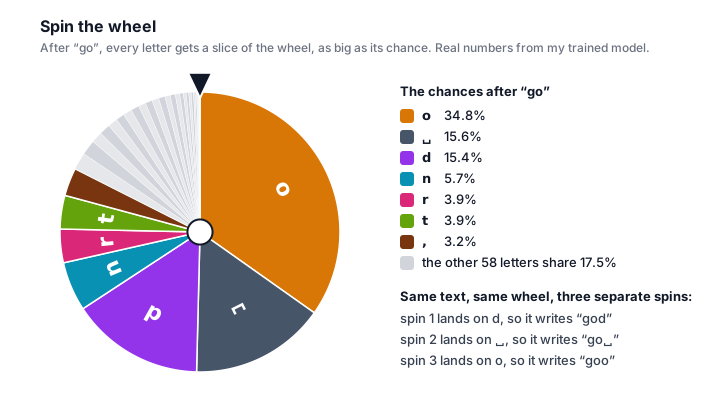
A good way to picture the second step is a prize wheel at a fair. The wheel has 65 slices, one for each letter that could come next, and each slice is as big as that letter's chance. After go, the model works out that o is the most likely next letter, so o gets the biggest slice: 34.8% of the way round the wheel. The space gets 15.6%, d gets 15.4%, and so on. To pick the next letter, spin the wheel, and write down whatever letter stops under the pointer.
 Scroll sideways, or tap the diagram to open it full size
The wheel after go, with the model's real chances. The same text gives the same wheel every time, but each spin can land somewhere different
In the example above the wheel often lands on the letter o. Sometimes it lands on a space. Now and then it lands on one of the thin grey slices, and that is what keeps the model's writing from being the same every time.
The wheel is not fixed. In this analogy the model works out a brand new wheel for every letter it writes, because every new letter changes the chances. An untrained model has slices that are all about the same size, so all it can write is noise.
Try it below. The text starts as go, the example above. Change it, and the model makes a new wheel; spin the wheel once to add one letter, or ten times in a row to watch the model write, one wheel at a time.
- Writing is the game played on repeat: guess a letter, write it down, stick it on the end, and guess again. Every line of "Shakespeare" this machine writes is produced one letter at a time, like that.
- Learning is the game too: guess, check the real answer, adjust, millions of times over. That is how the machine got good at the game, and it is the subject of the next post.
 Scroll sideways, or tap the diagram to open it full size
The guessing game, played three times in a row by my trained model, with its real chances. Each time, it gives every possible next letter a chance, picks one, and adds it to the end
That is the whole idea. Everything else in this post is detail about how the guessing is done.
Scores: what comes out of the closed box
Before the model can draw the wheel, it gives each of the 65 letters in its vocabulary a score: a plain number for how likely that letter is to come next. A score can be any size, even negative, and bigger means likelier. After go, o scores 4.878, the space 4.076, and d 4.062. The code calls these scores logits: one for each letter that could come next. What the logits really are, and how the model works them out from the text it is given, I come back to later; for now, I treat the model as a closed box that the scores come out of. One last step, softmax, turns the 65 scores into the 65 chances, the slices of the wheel. It always does this the same way. It makes every score positive, so even V, at −7.421, gets a slice, however thin. It keeps the scores in the same order, so the biggest score always gets the biggest slice. And it scales them so that the 65 chances add up to exactly 100%. Softmax: turning scores into chances, after temperature and top-k, shows the arithmetic. Two settings, temperature and top-k, can reshape the scores just before softmax, and the next two sections explain them.
None of these steps involves any luck. The model's scores, temperature, top-k, and softmax are all fixed arithmetic. Give my MiniGPT model the same text, and it gives exactly the same score (logit) for each letter that could come next, every time. Pass the same scores (logits) to the code that applies temperature, top-k, and softmax, with the same settings, and it makes exactly the same wheel of 65 chances (probabilities), one for each letter that could come next, every time. The only step that uses chance is the last one, the spin.
 Scroll sideways, or tap the diagram to open it full size
The model as a closed box. Temperature and top-k never touch what is inside it: they reshape the 65 scores that come out
Here is the wheel again, with the scores beside it. For the letters with the six biggest scores, the table shows every step: the score, the score divided by the temperature, whether top-k keeps it, and the chance that softmax gives it. The temperature and top-k sliders are explained in the next two sections; for now, leave them where they are.
Temperature: a bolder or a safer wheel
Before it spins, the model can reshape the wheel. A setting called temperature changes how big every slice is compared with the others. Turn it down, and the big slices grow and the thin ones shrink, so the model plays safe. Turn it up, and the slices even out, so the model takes more risks. Temperature is a hyperparameter: a setting that I choose, not something the model learned. Most hyperparameters, such as how many blocks the model has, are fixed before training, but temperature only changes how the wheel is spun, not how the chances are worked out, so it can be changed every time the model writes. Here is what it does to the wheel after go:
| Temperature | o | space | d | n | Letters under 2.5% share |
|---|---|---|---|---|---|
| 0.5, cautious | 68.0% | 13.6% | 13.3% | 1.8% | 5.1% |
| 0.8, the notebook's setting | 45.1% | 16.6% | 16.3% | 4.7% | 11.5% |
| 1, the wheel as it is | 34.8% | 15.6% | 15.4% | 5.7% | 17.5% |
| 2, bold | 13.7% | 9.2% | 9.1% | 5.5% | 37.5% |
Turn it all the way down to 0, and the model always takes the biggest slice, and writes the same text every time. Turn it right up, and every slice heads towards the same size, and the writing turns to noise. The full demo at the end lets you watch it on whole lines.
Temperature in the original Python
In Jibin Joseph's notebook, the writing loop, generate_text, takes temperature as a setting, with a default of 0.8. These are the notebook's own lines and comments:
PYTHON
1# Select logits from the last time step.
2logits = logits[:, -1, :]
3
4# Apply temperature scaling.
5logits = logits / temperature
The first line needs explaining. The closed box does not give out just one set of 65 scores. It gives one set for every letter of the text, up to 128 of them: one row of 65 scores for each position. Each row is the model's guess at the letter that comes after that position. For go, logits holds 2 rows:
| Row | The guess after | Biggest scores |
|---|---|---|
| 1 | g | space 3.830, e 3.261, o 3.025 |
| 2 | go | o 4.878, space 4.076, d 4.062 |
Only the last row is a guess about the letter that comes next, so logits[:, -1, :] keeps that row and drops the rest. The first : is the batch: the notebook can work on several texts at once, and here there is just one. The -1 picks the last row, and the final : keeps all 65 scores in it.
This might look wasteful, but it is just how the model works. The blocks have to work out a hidden state for every position anyway, because attention lets each letter look back at the ones before it. Scoring all of them costs a little extra while the model writes, but in training every row is useful: in practice text, the real next letter after every position is already known, so all of the guesses can be checked at once. The next post shows how.
That is all there is to it. After the first line, logits holds the 65 scores for what the next letter might be, and dividing it by one number divides every score by that number: 65 divisions in one line.
 Scroll sideways, or tap the diagram to open it full size
The temperature lines again, with a note beside each line in my own words
Here is what it does to the two biggest scores after go:
| Divide by | o | space | Gap | o's slice ÷ space's |
|---|---|---|---|---|
| 0.5 | 9.757 | 8.151 | 1.6 | 5 |
| 1 | 4.878 | 4.076 | 0.8 | 2.2 |
| 2 | 2.439 | 2.038 | 0.4 | 1.5 |
At temperature 1, o's slice (34.8%) is 2.2 times the space's (15.6%). At 0.5, it is 5 times as big (68.0% against 13.6%), and at 2, only 1.5 times (13.7% against 9.2%).
The gap is what matters. Softmax ignores the scores themselves and looks only at the gaps between them: how much bigger one letter's slice is than another's is e raised to the power of the gap between their scores. Dividing by 0.5 doubles every gap, so the favourite pulls further ahead. Dividing by 2 halves every gap, so the slices even out. Dividing by 1 changes nothing. As the temperature heads towards 0, the gaps grow without limit and the favourite takes the whole wheel; as it heads upwards, the gaps shrink towards nothing and every letter's slice heads towards 1 in 65.
A temperature of exactly 0 would make the notebook divide by zero. The demos on this page treat 0 as "always take the biggest slice" instead, which is where a temperature heading towards 0 is going anyway.
The name comes from physics, and it is more than a figure of speech. The same formula, called the Boltzmann distribution there, gives the chance of finding a particle at each energy level: e raised to the power of minus the energy, divided by the temperature, then scaled so that the chances add up to 1. A lower energy level is a likelier one, so a letter's score plays the part of minus the energy: a high score is like a low, comfortable level. When it is cold, almost every particle settles into the lowest level, like the favourite taking the whole wheel. When it is hot, they spread out across every level, like every letter getting a similar slice. As Wikipedia's softmax article puts it, "In statistical mechanics, the softargmax function is known as the Boltzmann distribution (or Gibbs distribution)."
Machine learning borrowed the word. In Distilling the Knowledge in a Neural Network (2015), Geoffrey Hinton, Oriol Vinyals, and Jeff Dean write softmax with a T in it, and explain:
T is a temperature that is normally set to 1. Using a higher value for T produces a softer probability distribution over classes.
A softer distribution is an evener wheel: exactly what the table above shows at a temperature of 2.
Top-k: keeping only the biggest slices
Even a good wheel has dozens of thin slices for letters that make no sense where they are. Usually the pointer misses them, but spin often enough and it will land on one, and a single nonsense letter can throw off everything written after it. One way to stop that is to trim the wheel before spinning it: keep only the k biggest slices, throw the rest away, and let the survivors share the whole wheel between them, each in proportion to its chance. This is called top-k.
Like temperature, k is a hyperparameter: a setting that I choose, which can be changed every time the model writes, with no retraining. Here is what it does to the wheel after go:
| Keep the biggest | o | space | d | n | Slices left |
|---|---|---|---|---|---|
| all 65 | 34.8% | 15.6% | 15.4% | 5.7% | 65 |
| 5 | 46.2% | 20.7% | 20.4% | 7.6% | 5 |
| 3 | 52.9% | 23.7% | 23.4% | 0 | 3 |
| 1 | 100% | 0 | 0 | 0 | 1 |
A small k makes the model play safe: with k = 1 it always takes the biggest slice, and writes the same text every time. A big k leaves room for surprises, good and bad.
Top-k in the original Python
In Jibin Joseph's notebook, the writing loop, generate_text, takes top_k as a setting, with a default of 200. It trims the wheel just before the chances are worked out, while they are still scores: one number per letter, where a bigger score means a bigger slice (lm_head: where do the 65 scores come from?, below, explains them). These are the notebook's own lines and comments:
PYTHON
1# Apply top-k filtering if requested.
2if top_k is not None:
3
4    # Keep no more than vocabulary size.
5    k = min(top_k, logits.size(-1))
6
7    # Find top-k logits.
8    values, indices = torch.topk(logits, k=k)
9
10    # Create filtered logits filled with -infinity.
11    filtered_logits = torch.full_like(logits, float("-inf"))
12
13    # Scatter top-k values into filtered logits.
14    filtered_logits.scatter_(dim=-1, index=indices, src=values)
15
16    # Replace logits with filtered logits.
17    logits = filtered_logits
torch.topk finds the k biggest scores and which letters they belong to. torch.full_like makes a fresh list of 65 scores, every one of them minus infinity, and scatter_ puts the k biggest scores back in their places. When softmax turns scores into chances, a score of minus infinity becomes a chance of exactly 0, so those slices vanish, and the survivors share the whole wheel.
 Scroll sideways, or tap the diagram to open it full size
The top-k lines again, with a note beside each line in my own words
Top-p: keeping slices up to a share
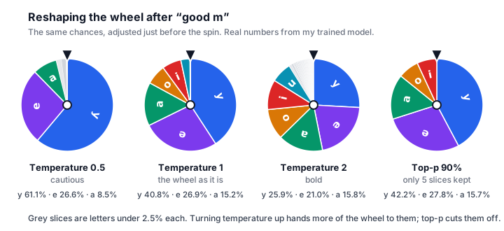
Top-k always keeps the same number of slices, however the chances are spread. A second way to trim the wheel adapts to the wheel itself: keep the biggest slices until they add up to a share p, and cut the rest. This is called top-p, or nucleus sampling. With p = 90%, my model's wheel after good m keeps just 5 slices: y, e, a, o, and i, which between them hold about 97% of the chance. The other 60 slices, which shared the remaining 3%, are cut away, and the 5 survivors are stretched to fill the whole wheel before the spin.
 Scroll sideways, or tap the diagram to open it full size
The real wheel after good m, reshaped by temperature and by top-p
The notebook has no top-p; the full demo at the end adds it as a slider. Temperature and trimming work together:
Softmax: turning scores into chances
Temperature and top-k reshape the scores. The last step, softmax, turns them into chances. Scores are not chances: they can be negative, and they do not add up to anything in particular. Softmax fixes both, in three moves:
- Take the biggest score away from every score. The biggest becomes 0, and every other score becomes negative. This keeps the numbers small, and it does not change the answer.
- Raise e to the power of each one. e is a number, about 2.718, and raising it to any power gives a positive number: e to the power 0 is 1, and e to a negative power is between 0 and 1. So every letter now has a positive number, and the bigger the score, the bigger the number.
- Divide each one by the total. Now the 65 numbers add up to exactly 1, or 100%: they are chances.
Here it is for go, at temperature 1 with all 65 letters kept. Once e is raised to the power of each one, all 65 add up to 2.874, so each chance is its own number divided by 2.874:
| Letter | Score | Minus 4.878 | e to that power | Chance |
|---|---|---|---|---|
o | 4.878 | 0 | 1.000 | 34.8% |
| space | 4.076 | −0.802 | 0.448 | 15.6% |
d | 4.062 | −0.816 | 0.442 | 15.4% |
n | 3.068 | −1.810 | 0.164 | 5.7% |
Those are the slices of the wheel after go.
Why e? Because it turns a gap between two scores into a ratio between two chances: one letter's chance divided by another's is always e raised to the power of the gap between their scores. o scores 0.802 more than the space, so its slice is e to the power 0.802, 2.2 times as big. That is why temperature works: dividing the scores changes the gaps, so it changes the ratios. And a score of minus infinity, which is what top-k gives the letters it cuts, becomes e to the power of minus infinity, which is 0: a chance of exactly 0.
Softmax in the original Python
In Jibin Joseph's notebook, softmax is one line in the writing loop, generate_text, straight after temperature and top-k. This is the notebook's own line and comment:
PYTHON
1# Convert logits into probabilities.
2probs = torch.softmax(logits, dim=-1)
torch.softmax does all three moves at once. dim=-1 tells it which way to add up: along the last dimension of logits, the 65 letters, so the 65 chances add up to 1.
Try temperature and top-k on the wheel
This is the wheel from the first demo, with the two settings added. Moving a slider reshapes the wheel straight away, before it spins, and the model's trained numbers stay exactly as they are.
Settings I cannot change: 65 letters and 128 positions
Temperature and top-k are hyperparameters I can change every time the model writes. Other things are fixed when the model is built, and they cannot change without training it again. Two of them matter already:
| What is fixed | Mine | What it decides |
|---|---|---|
| The vocabulary | 65 letters | which letters it knows: one score and one slice each |
The context length, block_size | 128 | the most letters it can look at at once |
The vocabulary is the set of letters the model knows: every different character in Tiny Shakespeare, which is capital and small letters, the space, the new line, and a few punctuation marks and other symbols. Each one has an ID number, from 0 for the new line to 64 for z. That is why there are 65 chances, and 65 slices on the wheel. The notebook's setting vocab_size is only how many letters there are; what is really fixed is which letters they are, and in which order. Every letter has its own row in two tables, its token embedding at the start of the model and its row of lm_head at the end, both found by its ID. A letter the model never trained on has neither, and swapping two IDs would hand each letter the other one's rows. The demos skip any character outside the vocabulary.
The 128 is the context length, or context window. When the text is longer than 128 letters, the model looks at the last 128 only, and anything further back is simply gone.
How much can it see at once?, later in this post, explains where the context limit comes from, and why raising it costs so much.
The real code: a list of 65 chances, and a spin
The wheel is only a picture, but the live demo below does something very close to it. Before it picks a letter, it has worked out a list of 65 chances, one for each letter that could come next, in the order of the letters' ID numbers (Letters to numbers explains the IDs). Here is that list after go, with the letters that matter, and a running total. The chances add up to exactly 1:
| ID | Letter | Chance | Running total |
|---|---|---|---|
| 0 | new line | 0.96% | 0.0096 |
| 1 | space | 15.59% | 0.1656 |
| … | |||
| 6 | , | 3.24% | 0.2080 |
| … | |||
| 42 | d | 15.38% | 0.4153 |
| … | |||
| 52 | n | 5.69% | 0.5308 |
| 53 | o | 34.80% | 0.8788 |
| … | |||
| 64 | z | 1.0000 |
In Jibin Joseph's notebook, the spin is one line. The notebook's writing loop, generate_text, holds the 65 chances in a PyTorch list called probs, and hands them to torch.multinomial, which picks one ID at random, each with its own chance: exactly what the wheel does. Then torch.cat adds the new ID to the end of the text so far, idx, ready to go round the loop again. These are the notebook's own lines and comments:
PYTHON
1# Convert logits into probabilities.
2probs = torch.softmax(logits, dim=-1)
3
4# Sample next token ID.
5next_id = torch.multinomial(probs, num_samples=1)
6
7# Append sampled token ID.
8idx = torch.cat([idx, next_id], dim=1)
Sample is the experts' word for spinning the wheel. The first line is softmax, turning the 65 scores into the 65 chances; just before it, the loop can also reshape the scores with temperature and top-k. Where the scores themselves come from is what the next section explains.torch.multinomial keeps the walk round the wheel hidden inside PyTorch, but what it does is simple. It picks a point somewhere round the wheel: a random number between 0 and 1. Then it walks round the wheel in ID order, slice by slice, adding up the chances, until it passes that point, and returns the ID of the slice it stopped in. If the random number is 0.6, the walk passes the new line, the space, the comma, d, and n (a running total of 0.5308), and stops inside o's slice, which runs from 0.5308 to 0.8788. So it returns 53, o. If the random number is 0.3, it stops inside d's slice instead, between 0.2080 and 0.4153. A big slice covers more of the numbers between 0 and 1, so it is picked more often: o about 35 times in every 100 spins.
 Scroll sideways, or tap the diagram to open it full size
The sampling lines again, with a note beside each line in my own words
torch.cat then adds the new ID to the end of idx, and when the text is shown, the notebook's decode turns each ID back into its letter. The vocabulary is the list of the 65 letters in ID order, so ID 53 becomes o. Where the list of chances comes from is what the rest of this post explains, layer by layer.
lm_head: where do the 65 scores (logits) for the next letter come from?
Until now, I have treated the model as a closed box: text goes in, and 65 scores, the logits, come out: one for each letter that could come next. Now I open the box, one level down. I pass the text into my MiniGPT model, and inside, it goes through these stages:
- Each letter becomes a list of 128 numbers: one list for the letter itself, learned in training, plus one for its position in the text. The code calls these the token embedding and the position embedding, and a later section explains them.
- The lists pass through four blocks, which let each letter's list take in what the letters before it say. The blocks are where the model does its understanding, and the four blocks explains them. Between blocks, each letter's list is called its hidden state: hidden, because nobody outside the model sees it.
- Out of the last block, after one final normalisation, comes the last letter's list: 128 numbers that sum up the text so far. This is the final hidden state, and the notebook's own comment calls it that.
lm_headturns the final hidden state into 65 scores, one for each letter that could come next. The code calls the scores logits.- Temperature and top-k reshape the scores, and softmax turns them into the 65 chances, or probabilities: the slices of the wheel. The sections above covered this stage.
 Scroll sideways, or tap the diagram to open it full size
The closed box from earlier, opened. The text and the 65 scores are the same; what is new is how the scores are made inside, ending with lm_head
Everything up to stage 3 is the body of the model. This section is about stage 4, lm_head, and the final normalisation just before it.
First, the final normalisation. Out of the last block come hidden states, one for each letter in the text: two for go. Only the last one matters here, because it is the only one that has seen the whole text. Its numbers are small: for go, they run from −1.26 to 1.00, and their spread, a measure of how far they typically sit from their average, is 0.33. The final normalisation, final_ln in the code, puts the list on a steady scale. First it rescales the 128 numbers so that they average 0 and spread 1. Then it stretches and shifts each number by its own trained amount. Its first four numbers go from −0.04, 0.17, 0.05 and −0.14 to −0.23, 0.70, 0.08 and −0.39. The pattern stays much the same, but now lm_head gets numbers on the same scale whatever the text was. The result is the final hidden state. The blocks use the same kind of normalisation inside them, which the four blocks comes back to.
Then lm_head scores each letter that could come next. lm_head, short for language-model head, is the model's last layer. It is a table with one row for each of the 65 letters. Each row holds 128 numbers, learned in training, plus one extra number, a bias: 8,385 numbers in all. To score a letter, lm_head multiplies the final hidden state by that letter's row, number by number, adds up the 128 results, and adds the bias. This multiply-and-add is called a dot product. A big score means the final hidden state looks like the letter's row, and training made each row look like the moments when that letter comes next. After go, o scores 4.878, the space 4.076, d 4.062, and n 3.068. The lowest of the 65 is V, at −7.421.
The bias: a head start for common letters. The bias is added whatever the text is, so it is a letter's starting score, before the final hidden state has any say. In my trained model the biases are tiny, from −0.107 for & to 0.057 for s, and they follow how common each letter is in Tiny Shakespeare: s, e, the space, and t get the biggest head starts, and &, $, 3, Q, and J the biggest handicaps. The dot product does almost all of the work: for o after go, it gives 4.845, and the bias adds just 0.033. The demo below shows both parts of every score.
It is called a head because it sits on top of the body. The body understands the text; the head reads the answer out in the form the task needs. Here the task is "which of 65 letters comes next?", so the head has 65 outputs. Nobody wrote the rows by hand: like every other number in the model, they started random, and training nudged them until the scores they give match what Tiny Shakespeare really does next.
Under the hood: When lm_head and the token embeddings share one table
In the notebook's bigger setup, with 384 numbers per letter, one line makes each letter's row of lm_head the very same list of numbers as its token embedding: model.lm_head.weight = model.token_embedding.weight. This trick, called weight tying, works because both tables have 65 rows of the same width, and it saves a whole table of numbers. GPT-2 does the same. My trained model does not: I checked, and its lm_head and its token embeddings are two separate tables, each learned on its own.
From there, the 65 scores go through temperature, top-k, and softmax, as the sections above showed. For go, at temperature 1, o's score of 4.878 becomes 34.8%, the biggest slice of the wheel.
Try it below. Type some text, and see what lm_head does with it: the final hidden state comes out of the blocks, and lm_head multiplies it by one letter's row, number by number, and adds up the results. Pick one of the six letters to see its sum. Then move the sliders.
In the original Python: lm_head
In Jibin Joseph's notebook, the final normalisation and lm_head are a line each. lm_head is one PyTorch layer, created in MiniGPT.__init__ as self.lm_head = nn.Linear(config.n_embd, config.vocab_size): a table of 65 rows of 128 numbers, self.lm_head.weight, plus 65 biases, self.lm_head.bias. nn.Linear is PyTorch's name for a layer that does dot products against a table of rows. At the end of MiniGPT.forward:
PYTHON
1# Final LayerNorm.
2x = self.final_ln(x)
3
4# Convert final hidden states into vocabulary logits.
5logits = self.lm_head(x)
In the code, the hidden states are just x, one list for each letter, all the way through the model.
 Scroll sideways, or tap the diagram to open it full size
The lm_head lines again, with a note beside each line in my own words
The scores are called logits. Then, in the writing loop, generate_text:
PYTHON
1# keep only the last row: the scores for the next letter
2logits = logits[:, -1, :]
3# the chances: the slices of the wheel
4probs = torch.softmax(logits, dim=-1)
self.lm_head(x) does the dot products for every hidden state and all 65 rows at once, and torch.softmax is the softmax step from earlier. The notebook scores every letter's hidden state, because training needs them all, and then keeps only the last letter's scores.
Four blocks in a row
One level further into the box. The final normalisation and lm_head read a hidden state, and that hidden state comes out of the biggest part of the model: four blocks, run one after another. This section is about what the blocks do as a whole; the sections after it open one up.
Going into block 1, there is one hidden state for each letter in the text, and each one knows only its own letter and its own position. (Where those starting hidden states come from is the last layer of the box, further in.) Each block has two parts: attention, where each hidden state looks back at earlier positions and collects information from them, and the MLP, a small network that works on each hidden state on its own. Every block reads the hidden states and rewrites them.
Attention followed by the MLP makes one block. My model runs four blocks in a row, and the bigger model in the notebook runs six. The blocks run one after another. The hidden states that come out of block 1 are the ones that go into block 2, block 2's go into block 3, and so on. After block 4, the final normalisation and lm_head read the last hidden state. Each block has its own parameters: the four blocks are built the same way, but they do not share any numbers, so each one can learn to do something different. With each block, the hidden states carry more context: by the later blocks, a hidden state is less about one letter and more about what is going on around it.
The hidden states that come out of one block and the ones that go into the next are not two different things: they are the same vectors, and in the code they are the same variable, x. A block never swaps a hidden state for a new one. It adds to it twice: hidden state out = hidden state in + what attention adds + what the MLP adds. Here is how much each block adds to hidden state 3 in goo, where "size" is how big its 128 numbers are taken together:
| Block | Size going in | Attention adds | The MLP adds | Size coming out | How alike in and out are |
|---|---|---|---|---|---|
| 1 | 0.50 | 0.59 | 1.66 | 2.16 | 0.47 |
| 2 | 2.16 | 0.80 | 0.85 | 2.72 | 0.90 |
| 3 | 2.72 | 0.90 | 1.16 | 2.92 | 0.90 |
| 4 | 2.92 | 0.74 | 1.86 | 3.09 | 0.78 |
Block 1 changes the hidden state the most: it adds more than the vector held when it went in. Blocks 2 and 3 refine it, so what comes out is still 0.90 like what went in. Block 4 makes a bigger change again, mostly in its MLP, as it gets the hidden state ready for lm_head. By the end, hidden state 3 scores only 0.08 for likeness to the vector it started as.
 Scroll sideways, or tap the diagram to open it full size
All the hidden states go through every block together. The coloured squares on each one show how much of the earlier positions it has taken in: hidden state 1 can only ever take in itself, while hidden state 3 takes in all three
Written out in full, the hidden states go through eight stages, always in the same order: attention, MLP, attention, MLP, attention, MLP, attention, MLP. The two take turns, and neither ever runs twice in a row. So if you see a diagram of a big GPT as a long stack of slabs labelled "Attention, Multilayer Perceptron, Attention, Multilayer Perceptron…", like the one in Grant Sanderson's talk, it shows exactly what my small model does. The only difference is how many times the pair repeats: GPT-3 repeats it 96 times, with much longer vectors.
Two details keep the blocks working well:
- Add, never replace. Each block adds to the hidden states rather than replacing them, so nothing learned in an earlier block is lost. This also matters for learning: when the parameters are tuned, the message about which way to turn them has to travel backwards through every block, as the next post shows. Adding rather than replacing gives that message a clear route all the way back, which is why models can be stacked dozens of blocks deep. Because every block adds to the same hidden states, they have another name in the jargon, taken together: the residual stream. It starts as the input embeddings and flows through every block.
- Normalise before each step. Before attention, and again before the MLP, the numbers in every hidden state are rescaled to a standard range, so that no position is shouting. Then each of the 128 numbers is stretched and shifted by its own two fixed parameters, set by training, so the machine can turn some numbers back up if they matter more than others. This is called layer normalisation, or LayerNorm.
Under the hood: How normalising works, with real numbers
Take hidden state 3 in goo as it arrives at block 1: the o token embedding plus the position 3 embedding. Its 128 numbers are tiny, between −0.104 and 0.111, and start 0.019, −0.080, 0.013. Normalising takes three moves:
- Subtract the average. The average of all 128 numbers is 0.0009, so here this barely changes anything.
- Divide by the spread. The numbers' typical distance from their average, their standard deviation, is 0.0444. Dividing by it gives the vector a standard size, whatever size it arrived at: its numbers now start 0.40, −1.83, 0.28, and run from −2.36 to 2.48.
- Stretch and shift. Each of the 128 numbers is multiplied by its own stretch, and has its own shift added: two parameters each, set by training. For the first three numbers, the stretches are 1.05, 1.12, and 1.08, and the shifts are 0.01, −0.03, and −0.08.
The result starts 0.43, −2.10, 0.22 (allowing for rounding): the numbers that go into block 1's weights in Where the queries, keys and values come from. MiniGPT (Part 5) tries a simpler kind of normalising, RMSNorm, which skips the first move and the shift.
Why four blocks, and not one? Because each block builds on the last. After block 1, a hidden state knows about the positions just before it. In block 2, it can look at hidden states that have already gathered their own neighbours, so it learns about positions further back, and so on. You can see this in the heads themselves. In block 1, the heads look between 1.6 and 5.7 positions back on average. In blocks 2 to 4, they look between 6 and 25 positions back.
You can also watch the guess improve. After each block, I took the last hidden state as it was at that point, gave it the same final normalisation, scored it against the same 65 rows of lm_head, and turned the scores into chances, exactly as the model does after block 4. lm_head was only ever trained to read block 4's output, so this is a peek rather than something the machine does when it writes, but it works surprisingly well, and researchers use the same trick under the name logit lens:
 Scroll sideways, or tap the diagram to open it full size
Real numbers from my trained model. Straight from the embeddings, before any block, it guesses the next letter right 12% of the time; after all four blocks, 49%
The picture follows the guess after Before we proceed any further, hear me spea, from the first speech in Tiny Shakespeare. Straight from the embeddings, before any block, the machine knows only that the last letter is an a, so it guesses y. Block 1 adds the letters in the positions just before it, and t takes the lead. Block 2 has seen enough of spea to try c. Only in blocks 3 and 4 does the whole picture, hear me spea, settle on k, at 98%.
Try it below. The text starts as the line in the picture above. Choose how many of the four blocks run, from none, where lm_head reads the hidden state straight from the embeddings, to all four, the real model.
The blocks in the original Python
In Jibin Joseph's notebook, the four blocks are a loop near the end of MiniGPT.forward:
PYTHON
1# the four blocks, in order
2for block in self.blocks:
3    # each one rewrites the hidden states
4    x = block(x)
self.blocks is an nn.ModuleList holding four TransformerBlocks, one for each of n_layer = 4, and each with its own fixed weights. Block 1's output is block 2's input, because it is literally the same variable.
Each block is a TransformerBlock, and its forward is two lines:
PYTHON
1# normalise, attention, add the result
2x = x + self.attn(self.ln1(x))
3# normalise, MLP, add the result
4x = x + self.mlp(self.ln2(x))
These two lines are a whole block. Read from the inside out, the first one normalises every hidden state (self.ln1, a layer normalisation), runs attention (self.attn), and adds what attention returns onto the hidden states (x + …). The second does the same with the MLP. The x + is "add, never replace", the residual connection. Normalising before each step, rather than after, is called pre-LayerNorm, and it tends to train more stably as models get deeper.
 Scroll sideways, or tap the diagram to open it full size
The blocks code again, with a note beside each line in my own words
Then the MLP: each hidden state on its own
Inside each block, after attention, every hidden state goes through the MLP, short for multilayer perceptron: a small two-layer network that works on each hidden state on its own. Every hidden state gets the same calculation, but each one sees only its own numbers. It is the simpler half of a block, so I open it first; attention, the half that looks back at other letters, comes next.
The MLP matters more than it sounds. About two-thirds of each block's parameters are in the MLP, rather than in attention.
So what is the MLP for? Grant Sanderson of 3Blue1Brown gives a good rule of thumb in his talk on transformers: where a guess needs context, attention supplies it, and where it needs general knowledge, the MLP supplies it. His example is a big word-level model completing "Michael Jordan plays the sport of". Basketball appears nowhere in the sentence, so it must come from knowledge stored in the parameters, and researchers at Google DeepMind found evidence that facts like this live mostly in the MLPs. In our small model the knowledge is humbler. Once attention has gathered that the word so far is thoug, knowing that h comes next is knowledge of English spelling, not something written in the earlier positions.
Try it below: switch the MLP off in any of the four blocks, and compare the chances, and the writing, with the real model. The text starts as Romeo, halfway through thought.
The MLP in the original Python
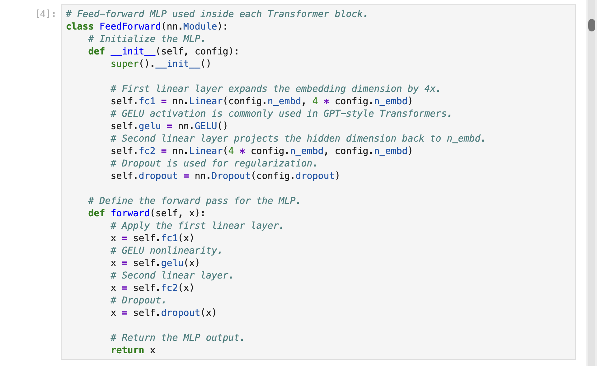
I ran the 1.3 cell, which defines the FeedForward class: two linear layers with a GELU between them, then dropout
PYTHON
1# 128 numbers → 512
2x = self.fc1(x)
3# bend: keep the positives, squash the negatives
4x = self.gelu(x)
5# 512 numbers → 128
6x = self.fc2(x)
The MLP works on each hidden state alone, using the same fixed weights for every position. fc1 and fc2 are nn.Linear layers, just like attention's, but fc1 makes 512 numbers from 128, giving the MLP room to look for many patterns at once, and fc2 brings them back to 128. gelu (Gaussian Error Linear Unit) is what makes the two layers more than one: without a bend between them, two weighted mixes in a row would be no more powerful than one. GELU passes large positive numbers through almost unchanged, pushes large negative numbers to about zero, and curves smoothly in between.
The MLP holds most of each block's numbers: 66,048 in fc1 and 65,664 in fc2, 131,712 in all, almost exactly twice attention's 66,048. It is the same kind of two-layer network as the digit reader in Machine Learning (Part 9).
 Scroll sideways, or tap the diagram to open it full size
The MLP code again, with a note beside each line in my own words
Inside a block: attention
Back to the first half of each block. Here is the problem attention solves. Take hidden state 3, the one that started as the last o in goo. It says "I am an o, in position 3". That is not enough to guess what comes next, because it says nothing about what came before. The same o could be the second o in good, in took, or in soon, and each of those wants a different next letter.
Here is a bigger example from Shakespeare itself. After a blank line, the next thing is almost always a speaker's name and a colon: in 7,219 of the 7,221 blank lines in Tiny Shakespeare. But there are 309 different speakers. Which name comes next depends on who has been talking in the scene, and that information is spread across all the positions before the blank line, not sitting in the one just before it.
So each block starts with attention, which has one strict rule: a hidden state may only look at hidden states in earlier positions, and at itself. Looking at later positions would be cheating, because the next letter is the answer it is trying to guess.
For attention, every hidden state makes three short-lived vectors, called its query, its key, and its value. The names come from searching: you type a query, it is matched against the keys, and you get back the matching values. It helps to picture them as cards at a meeting:
- The query says what this position is looking for in the earlier positions. Picture it as a card the position keeps in its own hand.
- The key says what this position has to offer. Picture it laid face up on the table, where its own position and every later position can read it.
- The value holds what this position will hand over if it is chosen. Picture it laid face down, next to its key.
Keys and values are separate because what makes a position worth listening to is not the same thing as what it should pass on. Then attention runs in three moves. Each hidden state:
- Matches its query against every key on the table from its own position or earlier.
- Shares out 100% of its attention, in proportion to how well each key matched.
- Collects that share of each value, adds them up number by number, and adds the result to itself.
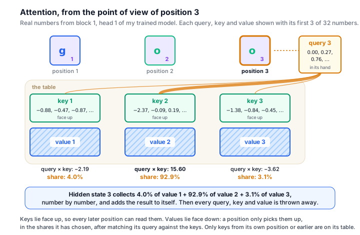
In block 1 of my trained model, in one of the four copies of attention that run side by side (heads, explained below), hidden state 3 gives 92.9% of its attention to position 2 (the first o), 4.0% to position 1 (the g), and 3.1% to itself, so most of what it collects is position 2's value.
 Scroll sideways, or tap the diagram to open it full size
Attention for position 3, the last position in goo. Its query matches position 2's key best, so most of what it collects comes from position 2's value
After this, hidden state 3 says something closer to "I am an o, and one position before me is another o". That is a much better clue, and the other heads add more, as you will see.
Where the queries, keys and values come from
The queries, keys and values are not looked up. A lookup table only works when there is a short list of things that can come in, one row for each: that is why token embeddings and position embeddings can be looked up, because there are only 65 letters and 128 positions. A hidden state can hold any 128 numbers at all, so no table could ever list them.
Instead, each block has three fixed tables of weights, one for queries, one for keys, and one for values. Each is a fixed grid of 128 × 128 numbers, called weights, plus 128 more fixed numbers, called biases. Training set them all, and while the machine is writing they never change, just like the token embeddings. In the code, each one is an nn.Linear layer, just like lm_head. To work out one number of a query, the machine multiplies each of the hidden state's 128 numbers by its own weight, adds up the 128 results, and adds a bias. It repeats that with a different row of weights for each of the query's 128 numbers. So every number of a query, key or value is a mix of all 128 numbers of the hidden state.
Here is one real number from my trained model: hidden state 3 in goo, at the start of block 1. The hidden state is normalised first, so it starts 0.43, −2.10, 0.22, and so on. The second number of its query is:
(−0.036 × 0.43) + (−0.038 × −2.10) + (0.030 × 0.22) + … 125 more terms … + 0.093 = 0.27
Three more things are worth knowing:
- The weights belong to the block, not to a position. Every hidden state goes through the same three tables of weights, so two hidden states that held the same numbers would make the same queries, keys and values. Each block has its own three tables, and between them they hold 49,536 of that block's parameters.
- They are all made at once. Making a position's query, key and value needs nothing but that position's hidden state, so the machine makes them for every position at the same moment, in one big multiplication over all the hidden states.
- They are thrown away. They exist only during attention. MiniGPT makes them all again from scratch for every new letter, because it reruns every position through every block. Big chatbots save that work. Because a hidden state only ever listens to earlier positions, adding a new letter never changes the hidden states before it, so their keys and values do not change either. Big models keep them instead of remaking them, in a store called the KV cache, short for key–value cache (this Hugging Face post explains it well). Only the newest position needs a new query.
Nobody chooses what goes into the queries, keys, and values. Training tunes the weights, just as it tunes the token embeddings, and a real model's queries and keys mostly have no tidy name at all.
Queries, keys and values, with real numbers
Here is attention for hidden state 3 in goo, with the real numbers from my trained model, in one of the four heads in block 1. In each head, each query, key and value is 32 numbers long; the heads section explains why. Hidden state 3's query starts 0.00, 0.27, 0.76, and so on. Matching a query with a key means multiplying the two together, number by number, and adding up the 32 results. A big total is a good match.
position 1 (g) | position 2 (o) | position 3 (o, itself) | |
|---|---|---|---|
| 1. Query × key, added up | −2.19 | 15.60 | −3.62 |
| 2. Divided by √32 | −0.39 | 2.76 | −0.64 |
| 3. Share of attention | 4.0% | 92.9% | 3.1% |
- Match. Multiply and add. That is all the "dot product" in the notebook is.
- Shrink. Divide by √32, about 5.66, to keep the scores in a modest range. Without this, the biggest score would swamp all the others.
- Share out. A step called softmax turns the scores into shares that are all positive and add up to 100%. The model uses the same trick again at the very end, to turn the final scores into chances.
- Collect. Hidden state 3 collects the values in those shares: 92.9% of position 2's, 4.0% of position 1's, and 3.1% of its own, number by number. After one more step, described under heads below, the result is added to hidden state 3.
Look at hidden states 2 and 3. They started from the same o token embedding. The only difference between them is their position embeddings, 2 and 3, and that is enough to give them different keys. Position 2's key matches the query with 15.60, while position 3's own key scores −3.62. Without the position embeddings, the machine could not tell "the o one position before me" from "me".
Try it below. Pick a block, a head, and a position, and follow its query through every step: matching it against each key, shrinking the scores, sharing out attention, and collecting the values. It starts on the example above: goo, block 1, head 1, position 3.
Attention in the original Python
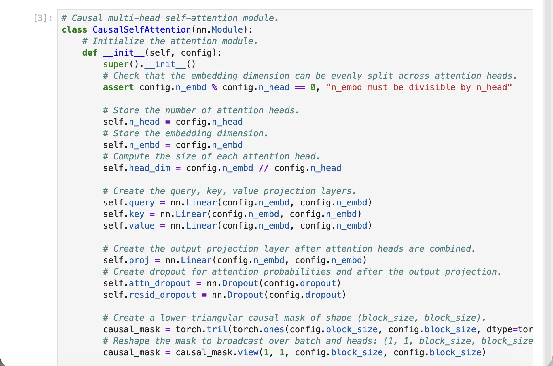
I ran the 1.2 cell. The top of the class, shown here, is __init__, which creates the weights and the causal mask
Like every part of the model, the class has two halves. __init__ runs once, when the model is built, and creates the fixed weights. forward runs every time, and uses them.__init__ creates four nn.Linear(128, 128) layers. Three of them are the tables of weights from Where the queries, keys and values come from: self.query, self.key, and self.value. The fourth, self.proj, mixes the four heads' results at the end. Each holds a 128 × 128 grid of weights and 128 biases, 16,512 numbers, so attention holds 66,048 in all. __init__ also builds the causal mask, the "only earlier positions" rule, as a triangle of True and False values. It stores the mask with register_buffer, so the mask is saved with the model, but training never changes it.
 Scroll sideways, or tap the diagram to open it full size
The mask, drawn out for eight positions. Each row is a position; the filled cells are the positions it may listen to
Then forward runs attention, in three stages. First, it makes the queries, keys, and values:
PYTHON
1# 1 text, 3 hidden states, 128 numbers
2B, T, C = x.shape
3# a query for every hidden state
4q = self.query(x)
5# a key for every hidden state
6k = self.key(x)
7# a value for every hidden state
8v = self.value(x)
9# cut each one into 4 pieces of 32
10q = q.view(B, T, self.n_head, self.head_dim)
11k = k.view(B, T, self.n_head, self.head_dim)
12v = v.view(B, T, self.n_head, self.head_dim)
13# group the pieces by head
14q = q.transpose(1, 2)
15k = k.transpose(1, 2)
16v = v.transpose(1, 2)
self.query(x) applies the query weights to every hidden state at once: each of the 128 numbers of each query is a weighted mix of all 128 numbers of its hidden state, plus a bias. view cuts each 128-number vector into four 32-number pieces, one per head, and transpose(1, 2) regroups them so that each head gets its own stack of pieces and all four heads can run side by side.
Second, it matches and shares out:
PYTHON
1# match every query with every key
2scores = q @ k.transpose(-2, -1)
3# shrink: divide by √32
4scores = scores / math.sqrt(self.head_dim)
5# the corner of the mask for 3 positions
6mask = self.causal_mask[:, :, :T, :T]
7# no listening to later positions
8scores = scores.masked_fill(mask == False, float("-inf"))
9# share out 100% of attention
10attn = F.softmax(scores, dim=-1)
q @ k.transpose(-2, -1) is the dot product between every query and every key, in one go: for each head, a 3 × 3 grid of scores. For hidden state 3 in head 1 of block 1, the row is −2.19, 15.60, and −3.62, the numbers from Queries, keys and values, with real numbers. masked_fill writes minus infinity into every score for a later position, and softmax turns minus infinity into exactly 0, so later positions get no attention at all. attn holds the shares: 4.0%, 92.9%, and 3.1% in that row.
Third, it collects and puts the heads back together:
PYTHON
1# collect the values, in those shares
2out = attn @ v
3# rejoin the four heads: 128 numbers again
4out = out.transpose(1, 2).contiguous().view(B, T, C)
5# mix what the four heads found
6out = self.proj(out)
7return out
attn @ v is the collecting: each hidden state's share of every value, added up number by number. The next line undoes the cutting into heads (I have joined three of the notebook's lines into one), and self.proj mixes the heads' findings. The result has the same shape as the hidden states, 1 × 3 × 128, which is what lets TransformerBlock add it straight back onto x.
 Scroll sideways, or tap the diagram to open it full size
The heart of attention, with a comment beside each line
Several heads at once
A block does not run attention just once. It runs it four times side by side, and each copy is called a head. Each head gets its own 32-number piece of every query, key, and value, and every piece is made from the whole hidden state. Same hidden states, same moment, but four different queries, and so four different answers.
Here is what hidden state 3 collects from each of block 1's four heads:
| Head | position 1 (g) | position 2 (o) | position 3 (itself) | In short |
|---|---|---|---|---|
| 1 | 4.0% | 92.9% | 3.1% | one position back |
| 2 | 83.4% | 12.2% | 4.4% | two positions back |
| 3 | 83.4% | 14.9% | 1.6% | two positions back |
| 4 | 24.7% | 66.5% | 8.8% | one position back, more loosely |
Between them, the four heads tell hidden state 3 exactly what it needs to know. Heads 1 and 4 say "one position back, there is an o", and heads 2 and 3 say "two positions back, there is a g". Put together: g, o, then me. That is goo, and it is why d ends up so likely.
The same habits show up on any text. Here are all four heads reading a line from Romeo and Juliet:
 Scroll sideways, or tap the diagram to open it full size
Real attention, measured from my trained model. Each row is a position, labelled with the letter it started from, and each dot shows how much attention it gives the position above
Nobody designed these habits. Training grew them, because they help with the guessing game. Two heads even learned nearly the same habit: nothing forces heads to be different, and training simply found two copies useful. Between them, after block 1, every hidden state carries information about the two or three positions before it, which is the same clue you would get by counting which letters follow which, and then some.
At the end of attention, what the four heads collected, 32 numbers each, is laid side by side to make 128 numbers again. One more table of weights then mixes them, so that what all four heads found ends up in the one hidden state.
Why 32? The machine makes one query, one key, and one value for each hidden state, each 128 numbers long and each made from the whole hidden state. Then it cuts each of them into four pieces of 32, one piece per head. So the heads share the block's three tables of weights between them, rather than each adding more. The 4 is not fixed. With 8 heads, each head's query, key, and value would be 16 numbers long: more queries, but cruder ones. The bigger model in the notebook uses 6 heads of 64. More heads is not automatically better; it is a trade-off that model builders settle by experiment. The only rule is that the vector size must divide evenly by the number of heads.
Try it below. Switch any of the 16 heads off, and compare the chances, and the writing, with the real model. A head that is off still works out its attention, but adds nothing to the hidden states. The text starts as goo.
Heads in the original Python
The heads are not separate pieces of code. The notebook makes one query, one key, and one value of 128 numbers for each position, then cuts each one into four pieces of 32 and regroups the pieces by head, so that all four heads run at once in the same multiplications. These lines are in the attention code above:
PYTHON
1# cut each one into 4 pieces of 32
2q = q.view(B, T, self.n_head, self.head_dim)
3# group the pieces by head
4q = q.transpose(1, 2)
and, after collecting the values, the reverse:
PYTHON
1# rejoin the four heads: 128 numbers again
2out = out.transpose(1, 2).contiguous().view(B, T, C)
3# mix what the four heads found
4out = self.proj(out)
 Scroll sideways, or tap the diagram to open it full size
The head lines again, with a note beside each line in my own words
Token embeddings and position embeddings
One level further in: where do the hidden states that go into block 1 come from? This is the model's first step. Each letter in the text has an ID number, which the last layer, below, explains; for now, it is enough that g is 45 and o is 53. Each ID picks a row from a table. The table has one row for each of the 65 letters, and each row holds 128 numbers: the machine's starting point for that letter. This row is the letter's token embedding, and a list of numbers like this is called a vector. It helps to picture the table as a box of flashcards, like the alphabet cards preschoolers learn from. The front shows the letter. On a preschool card, the back would say "a is for apple", with a picture. Here, the back holds the 128 numbers. In my trained model, the g token embedding begins −0.049, 0.032, 0.014, 0.030, and carries on for another 124 numbers. The next post shows where those numbers came from. Every lowercase o gets exactly the same token embedding, with the same 128 numbers, wherever it appears. A capital O gets a different one.
There is no limit on copies: goo simply looks up the o row twice. There is a row for every capital and every lowercase letter, because to the model G and g are completely different letters. On top of those 52, there are 13 more: the space, the new line, ten punctuation marks, and the digit 3. That last one is only there because the text labels 27 speeches 3 KING HENRY VI, so the table includes a whole row for a letter that appears just 27 times in 1.1 million.
 Scroll sideways, or tap the diagram to open it full size
Each token embedding pictured as a flashcard: the letter on the front, and its 128 real numbers on the back
Three things to know about these numbers:
- The numbers are fixed. In a trained machine, every token embedding is as good as printed in ink. The
grow has exactly the same 128 numbers every time agappears, in every piece of text, today and tomorrow. Writing, chatting, and answering questions never change a single one of them. The only way to change them is to train the machine again. - Nobody wrote them. There is no "number 7 is how vowel-like this is". None of the 128 numbers has a name.
- Training chose them. Every fixed number in the machine is called a parameter: all 826,433 of them in my small model. I picture each one as a dial, and training is what turned each dial to where it is now. How it settled on these exact numbers is the subject of the next post. In this post, the parameters are simply given, like a printed set of flashcards that I can copy as often as I like.
There is also a table of position embeddings. Picture the text as a row of numbered positions: position 1, position 2, and so on, with one vector for each position. This time, one of each is enough: a text might need a dozen copies of the o row, but my machine only ever needs the same 128 position embeddings, because a text never has two position 1s. Every letter takes the next position, whether it was in the text the machine was given or the machine has just written it, and its token embedding is combined with that position's embedding. Position embeddings work just like token embeddings: each one is 128 numbers, fixed by training in exactly the same way, so the two can be combined by simply adding them, number by number. So once a letter is placed on a position, the machine knows both what the letter is and where it sits. The position embedding is the only thing that tells the two os in goo apart at this stage.
 Scroll sideways, or tap the diagram to open it full size
Each position embedding pictured as a card: the position number on the front, and its 128 real numbers on the back
Here is the real g token embedding, the real position 1 embedding, and what they add up to:
 Scroll sideways, or tap the diagram to open it full size
Adding them is plain addition, number by number. The result depends on both the letter and its position
Adding each token embedding to its position embedding gives every position its starting vector, called its input embedding. For goo there are three: position 1 starts as the g embedding plus the position 1 embedding, position 2 as the o embedding plus the position 2 embedding, and position 3 as the o embedding plus the position 3 embedding. The blocks then rewrite these vectors, and from then on each one is called a hidden state: one for each position.
This is the last time the machine looks at letters. From here on, everything happens to the hidden states. The token and position embeddings are not touched again: they stay fixed, ready for the next text.
Under the hood: All 128 numbers in the g token embedding
These are the exact numbers in my trained model, rounded to three decimal places, eight to a row. The colours in the pictures above are these numbers: blue for those above 0, orange for those below.
CODE
1 -0.049,   0.032,   0.014,   0.030,   0.005,   0.005,  -0.015,   0.020
2  0.033,  -0.008,   0.028,   0.008,  -0.024,  -0.012,   0.037,   0.020
3  0.059,  -0.035,  -0.010,  -0.036,  -0.026,   0.029,  -0.062,  -0.032
4 -0.001,  -0.005,  -0.022,  -0.061,   0.015,  -0.031,  -0.060,   0.017
5 -0.029,   0.041,  -0.008,  -0.033,  -0.025,  -0.016,  -0.040,  -0.032
6 -0.043,  -0.030,  -0.035,   0.025,   0.018,  -0.079,  -0.078,   0.047
7 -0.002,   0.010,   0.071,  -0.008,  -0.036,   0.082,  -0.029,   0.040
8  0.036,   0.051,  -0.024,  -0.028,   0.005,   0.014,   0.004,  -0.010
9 -0.009,  -0.097,  -0.115,  -0.042,  -0.081,   0.051,   0.032,   0.015
10  0.000,  -0.059,  -0.002,   0.051,   0.024,   0.026,   0.006,   0.017
11 -0.019,  -0.007,  -0.002,  -0.012,   0.058,  -0.008,   0.001,  -0.041
12  0.069,  -0.027,  -0.036,   0.016,   0.070,  -0.012,  -0.026,  -0.015
13 -0.036,   0.067,  -0.054,  -0.028,  -0.047,  -0.029,   0.004,   0.005
14  0.022,  -0.028,   0.024,   0.032,   0.041,   0.006,   0.007,   0.063
15 -0.019,  -0.031,  -0.011,   0.030,  -0.053,  -0.007,  -0.001,   0.014
16 -0.003,   0.006,   0.025,   0.020,   0.009,   0.011,   0.082,   0.065
In the notebook, the two tables are token_embedding and position_embedding.
How many position embeddings there are is fixed in advance, when the machine is built. There is one for each position, and the number of positions is the most letters the machine can look at when it chooses the next letter. That limit is called the context length, and in the notebook it is block_size. I come back to it, and what it costs to raise it, in How much can it see at once?
Under the hood: How the position embeddings relate to each other
On its own, one position embedding looks as meaningless as a token embedding. The interesting part is how they relate to each other:
 Scroll sideways, or tap the diagram to open it full size
The bright diagonal shows that neighbouring positions ended up with similar embeddings. Nobody arranged that: training did
On average, the embeddings for neighbouring positions score 0.65 for how alike they are, where two random vectors would score about 0. Positions far apart point the opposite way: embeddings 100 positions apart score −0.35. So without being told, the machine turned its position embeddings into a kind of ruler, where "position 41" feels close to "position 42" and far from "position 120". That is just the kind of information attention needs, to find "the hidden state one position before me".
Try it below. Pick any letter in the text, and see its token embedding and its position embedding add up to the input embedding that block 1 receives.
Embeddings in the original Python
PYTHON
1# 1 text, 3 letters
2B, T = idx.shape
3# the positions: 0, 1, 2
4pos = torch.arange(0, T)
5# look up a token embedding for each ID
6tok_emb = self.token_embedding(idx)
7# look up a position embedding for each position
8pos_emb = self.position_embedding(pos)
9# add them: the input embeddings, the first hidden states
10x = tok_emb + pos_emb
These are the first lines of MiniGPT.forward, before the blocks. Python counts from 0, so position 1 in this post is row 0 in the code.self.token_embedding is the table of token embeddings. The model's __init__ creates it as nn.Embedding(config.vocab_size, config.n_embd): a table with 65 rows, one per letter, and 128 columns. Looking up an embedding is picking a row: g picks row 45, and both os pick row 53. self.position_embedding is the same kind of table, nn.Embedding(config.block_size, config.n_embd), with one row per position. Before training, __init__ fills both tables with small random numbers, with a standard deviation of 0.02, and training then tunes them.
 Scroll sideways, or tap the diagram to open it full size
Each letter's ID picks one row of the table, and that row's 128 numbers become the letter's token embedding. Both copies of o get the same row
x = tok_emb + pos_emb is where the hidden states are born. x holds one hidden state per position, 128 numbers each, and from here to the end of forward, x is the hidden states. The code never makes a new variable for them: every block overwrites x.
 Scroll sideways, or tap the diagram to open it full size
The embedding lines again, with a note beside each line in my own words
Letters to numbers
The last layer of the box, and the first thing the model does. Computers need numbers, so each of the 65 letters in the vocabulary gets an ID: its place in the list of all 65, sorted into the computer's standard order. In Tiny Shakespeare, g is 45, o is 53, and d is 42, so goo becomes [45, 53, 53]. That is all this step does. But an ID is just a name tag. 53 is not "more" than 45 in any way that helps, so the model cannot do much with the ID itself. That is why the very next step swaps each ID for its token embedding, as the layer above showed.
Try it below. Type anything, and watch each letter become its ID.
Letters to numbers in the original Python
In Jibin Joseph's notebook, the vocabulary and the IDs are built from the text itself, in section 2.2. These are the notebook's own lines and comments:
PYTHON
1# Sorted list of unique characters in the dataset.
2chars = sorted(list(set(text)))
3
4# Dictionary that maps each character to an integer token ID.
5stoi = {ch: i for i, ch in enumerate(chars)}
6
7# Dictionary that maps each integer token ID back to a character.
8itos = {i: ch for i, ch in enumerate(chars)}
9
10# Encode a string into a list of integer token IDs.
11def encode(s):
12
13    # Convert each character in the string into its integer ID.
14    return [stoi[ch] for ch in s]
set(text) keeps one copy of each different character in all 1.1 million letters of Tiny Shakespeare, and sorted puts them in order: 65 of them. stoi, "string to integer", looks up a letter's ID, and itos goes back the other way, which is how the model's IDs become text again when it writes. encode would stop with an error on a character that is not in the vocabulary; the demos on this page skip it instead.
 Scroll sideways, or tap the diagram to open it full size
The vocabulary code again, with a note beside each line in my own words
That is the bottom of the box. Starting from the outside, I have opened every layer: the wheel, the scores, lm_head, the four blocks, the MLP, attention, the heads, the embeddings, and now the IDs. There is nothing left inside that this post has not shown, in plain words, in a demo you can try, and in the notebook's Python.
The five steps
That is every layer, from the outside in. Here they are the other way round, in the order the model runs them: every time it writes one letter, it goes through the same five steps.
 Scroll sideways, or tap the diagram to open it full size
The five steps. Plain names in black; the names you will meet in the notebook in grey
Here are all five at once, for goo, with the real numbers from my trained model:
 Scroll sideways, or tap the diagram to open it full size
The whole journey for goo, with the real numbers from my trained model
Putting it together: choosing the next letter
Here is the whole journey once more, step by step, for choosing the next letter after goo. The two tables of embeddings are only the start. Almost everything that matters happens in the blocks.
- Look up. For each letter written so far, in order (
g,o,o), add its token embedding to its position embedding. That gives one input embedding per position. - Run four blocks. Each block is attention followed by the MLP, and every block rewrites every hidden state. By the end, each hidden state carries a mix of the earlier positions, so hidden states 2 and 3, which both started from an
o, are now very different. - Read only the last hidden state. It started as just the final
o, but after four blocks its numbers stand for the whole ofgooso far. - Turn it into chances. The machine scores the last hidden state against the 65 rows of
lm_head, one for each letter. That is one more fixed, learned table, 65 rows of 128 numbers each. The better the match, the bigger the chance. The 65 chances add up to 100%. - Spin the wheel, and write down whatever letter stops under the pointer. Almost every time, it is
d. - Repeat. Add the
dto the end of the text, look up its embeddings, and go back to step 2 withgood. The notebook really does rerun all the blocks on every position for every new letter.
Try it: my trained machine, running in your browser
Everything at once. This is my MiniGPT model itself, all 826,433 numbers of it, running in this page. Nothing is sent anywhere: the five steps happen on your own computer. Type anything, and watch the chances for the next letter change as you type. Then spin the wheel, or let it write 200 letters. Use the sliders to try temperature and the wheel trimming, and use the block and head buttons to look inside any of its 16 attention heads.
How much can it see at once? The context limit
My machine can see at most 128 letters at a time. That limit is called the context length, or context window, and in the notebook it is block_size. Anything further back than 128 letters is simply gone: the machine has no idea it was ever there.
The limit comes from the position embeddings. There is one for each position, and there are 128 of them, so there is no position 129 to put a letter on.
So why not simply give the machine thousands of positions? Because seeing further costs more in four ways:
- More to learn. Every extra position needs its own position embedding, and it has to be learned in training like every other parameter. The practice snippets have to be as long as the row, too, so that the machine actually practises using the far positions.
- Much more expensive attention. In attention, every hidden state matches its query against the key of every earlier position. Twice as many positions means about four times as many checks, and four times as much memory for the grid of attention. Ten times the positions means about a hundred times the checks.
- Slower writing. Every new letter is chosen by running the whole row through all four blocks, so a longer row makes every single letter slower to write.
- Seeing is not the same as using. A machine with more positions only gets better if it learns to use the far-away letters, and that needs practice text where letters far back really matter.
This is the same limit you meet in chatbots, where it is called the context window and counted in tokens rather than letters. Today's models can see hundreds of thousands of tokens at once. They get there partly with better ways of marking positions than a fixed table of position embeddings, like the rotary position embeddings I tried in MiniGPT (Part 5), and partly with cheaper kinds of attention, like the windowed attention in MiniGPT (Part 7). Windows are usually mixed with some blocks of full attention, because, as Part 7's secret-word test shows, a window does not reach further back on its own.
Beyond the guessing game: tools, harnesses, and agents
A GPT can only guess the next piece of text, yet chatbots check the weather, read files, and run programs. The trick is that the model writes a request, such as {"tool": "get_weather", "location": "NYC"}, and an ordinary program around it, the harness, spots the request, carries it out, and adds the result to the text, so that the model carries on guessing with the answer in front of it. The model never runs anything itself; it only ever writes text, and models learn to write these requests in a later stage of training, covered in the next post. An agent is what you get when a harness lets the model keep that loop going by itself, for many steps, towards a goal. My MiniGPT could not do any of this: it never saw a request, and 128 letters is far too short to hold one. I wrote more about organising agents in Agent Orchestration, and about plugging tools into a harness in Model Context Protocol.
Why the big models do not use letters
Back at the start, I asked why the big models do not guess one letter at a time. There are three reasons, and attention explains the first one:
- The rows get longer, and attention gets much more expensive. A piece of a word is about four letters of English on average, so the same text needs about four times as many positions if every letter has its own. In attention, every position checks every position before it, so four times the positions means about sixteen times the checks.
- The early blocks waste their time spelling. With letters, the first blocks have to assemble
t,h,o,u,g,h,tinto a word before any meaning can start to build up. With a token embedding for the whole word, the meaning is there from the start. - But the pieces cannot be too big, either. A token for every whole sentence would be useless: most sentences turn up only once, so their embeddings could never be tuned. Words and pieces of words are the balance.
In MiniGPT (Part 3), I swap MiniGPT's letters for pieces of words to see what difference it makes.
We know the rules, not the result
Everything in this introduction (the embeddings, attention, the MLP, the wheel) is a calculation that can be written down exactly. The notebook does all of it in a few hundred lines. What nobody can write down is what the trained parameters mean. Nobody chose them: they grew. Working out what a trained model has actually learned is a research field of its own, called interpretability, and for big models it is mostly unsolved. In that sense a language model really is a black box: not because the machinery is secret, but because what the machinery learned was never written down by anyone. Here is one small peek inside.
A peek inside: which letters end up alike?
Nobody tells the machine that A and a are the same letter, or that a full stop and a question mark do a similar job. So once training has tuned the token embeddings, which ones end up looking alike? I compared every letter's token embedding in my trained model with every other letter's. A score of 1 would mean two embeddings carry identical numbers, 0 means they are unrelated, and a negative score means they point opposite ways.
| Letter | The letters whose embeddings are most like it |
|---|---|
a | A (0.50), then $, E, u, o |
t | T (0.61), then d, w, , |
q | Q (0.71), then J, j |
, | ; (0.83), then !, :, ? |
. | ? (0.83), then ! (0.80) |
| space | - (0.31), then the new line (0.30) |
Three things jumped out at me:
- Capital and lowercase letters pair up. Across all 26 letters, a capital and its lowercase letter score 0.46 on average, while two letters picked at random score about 0. The machine worked out for itself that
Aandaare, in some sense, the same letter. - Punctuation splits into two families. The comma sits right next to the semicolon (0.83), with the colon nearby: marks that mean "pause". The full stop sits next to the question mark (0.83) and the exclamation mark (0.80): marks that mean "this sentence is over".
- The vowels are a weaker family. Vowels' embeddings are only slightly alike (0.14 on average), and slightly unlike the consonants (−0.06). Look at the
arow above: apart from an odd$, the embeddings most likeaare other vowels'.
Here are all 65 token embeddings on one map, squashed from 128 numbers down to 2 so they fit on a page:
 Scroll sideways, or tap the diagram to open it full size
The punctuation marks gather on the right, the vowels drift towards the top, and most capitals sit on the left. The pairing of capitals with their lowercase letters does not survive the squash, but it is there in the full 128 numbers
None of this was programmed in. The only instruction the machine was ever given was to get better at guessing the next letter, and these families of letters are what that instruction grew. The next post shows how.
The jargon decoder
The terms for the whole series are collected in one table, the series glossary.
Here is each idea from this introduction in plain words, next to its name in the code and in papers. I come back to each one as the notebook reaches it. The words for how the machine is trained are in the next post.
| In plain words | What the experts call it |
|---|---|
| the guessing game | next-token prediction, or language modelling |
| a letter: any of the 65 symbols, even the space and the comma | a character |
| the thing being guessed: a letter here, a word or piece of a word in big models | a token |
| the 65 letters | the vocabulary |
| the chances for each possible next letter | a probability distribution, produced by a softmax |
| a letter's row of 128 learned numbers | its token embedding (token_embedding): a vector |
| a position's row of 128 learned numbers | the position embedding (position_embedding) |
| a token embedding plus its position embedding, before block 1 | the input embedding |
| the number of positions: how many letters it can see at once | the context length, or context window (block_size) |
| "only look at earlier positions" | the causal mask |
| what attention matches and collects | the query, the key, and the value vectors |
| the three tables of weights that make them | the query, key, and value projections (self.query, self.key, self.value) |
| keeping the keys and values instead of remaking them | the KV cache |
| add, never replace | the residual connection |
| the hidden states, as every block adds to them | the residual stream |
| a position's vector after a block | a hidden state |
| normalising a hidden state before attention and before the MLP | layer normalisation, or LayerNorm |
| every fixed number that training set | the parameters, or weights |
| spinning the wheel of chances | sampling |
| keeping the biggest k slices | top-k sampling |
| keeping the biggest slices until they add up to p | top-p, or nucleus, sampling |
| the 65 rows that score each letter that could come next | the language-model head (lm_head), or output layer |
| the scores, before softmax | the logits |
| a request the model writes for a program to carry out | a tool call, or function call |
| the program around the model | the harness |
| a harness letting the model act by itself for many steps | an agent |
| working out what the trained parameters mean | interpretability |
Opening the notebook
The repository is github.com/jibin10/MiniGPT. The README's recommended path is Colab: click the "Open in Colab" badge, select a GPU runtime (a computer with a graphics chip, a GPU, which does this kind of arithmetic much faster than an ordinary processor), and run the cells top to bottom. The notebook is designed to work that way with no local setup at all, but the only dependencies are torch, matplotlib, and requests, so running it on my own hardware was just as easy:
BASH
1git clone https://github.com/jibin10/MiniGPT.git && \
2cd MiniGPT && \
3python3 -m venv .venv && \
4source .venv/bin/activate && \
5pip install -r requirements.txt jupyter && \
6jupyter notebook MiniGPT_Notebook.ipynb
The commands are joined with &&, so they paste into a terminal as one command, and the chain stops at the first step that fails.
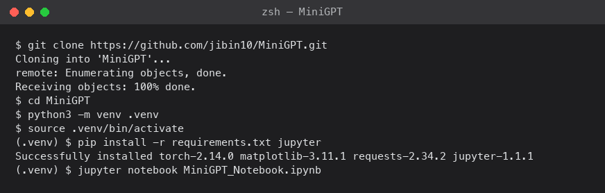
I cloned the repository and installed the three dependencies plus Jupyter into a fresh virtual environment
Notebook part 1: a minimal GPT model
The notebook comes in parts of its own, and builds the model before it loads any data. Its part 1 defines every piece of a small GPT (the embeddings, attention, the MLPs, and the final step that turns a hidden state into chances) and checks that a batch of random letters passes through it.
Here is how those pieces fit together, next to the digit-reading network from Machine Learning (Part 9). That network was two dense layers in a row: tables of weights of the same kind as this post's, where every number that comes out is a weighted mix of every number that goes in. MiniGPT's MLP is exactly that kind of two-layer network. Attention is the new part, slotted in front of it. Four of those blocks are stacked, and one more dense layer at the end, lm_head, turns each hidden state into 65 chances for the letter after it.
 Scroll sideways, or tap the diagram to open it full size
The MLP inside every MiniGPT block is the same kind of two-layer network as my MNIST digit classifier. What is new is the attention step in front of it
One thing helped me read the code. The notebook's Python is the blueprint for the machine: it says what shape every vector and table is, and how they are combined. It does not contain a single trained number. Run it untrained and you get the same machine, filled with random numbers. The trained numbers live in a separate file that training writes out, a checkpoint. For my exhibit it is exhibit.pt, 3.4 MB of named lists of numbers, and you can download it: Run my model yourself shows how. The live demo in this post runs the same numbers, copied into a file called weights.bin.
Under the hood: Where every fixed number lives
Every fixed thing in this post is one named entry in the checkpoint. The names come from the notebook's code, and the four blocks each have their own copy of the block entries, named blocks.0 to blocks.3.
| In this post | Name in the checkpoint | Shape | Numbers |
|---|---|---|---|
| the token embeddings | token_embedding.weight | 65 × 128 | 8,320 |
| the position embeddings | position_embedding.weight | 128 × 128 | 16,384 |
| in each of the 4 blocks: | |||
| normalise before attention | ln1.weight, ln1.bias | 128 + 128 | 256 |
| the query weights | attn.query.weight, attn.query.bias | 128 × 128 + 128 | 16,512 |
| the key weights | attn.key.weight, attn.key.bias | 128 × 128 + 128 | 16,512 |
| the value weights | attn.value.weight, attn.value.bias | 128 × 128 + 128 | 16,512 |
| mixing the four heads' results | attn.proj.weight, attn.proj.bias | 128 × 128 + 128 | 16,512 |
| normalise before the MLP | ln2.weight, ln2.bias | 128 + 128 | 256 |
| the MLP | mlp.fc1 (128 → 512) and mlp.fc2 (512 → 128), weights and biases | 131,712 | |
| after block 4: | |||
| the final normalisation | final_ln.weight, final_ln.bias | 128 + 128 | 256 |
the rows of lm_head | lm_head.weight | 65 × 128 | 8,320 |
lm_head's biases | lm_head.bias | 65 | 65 |
| total | 826,433 |
What is not in the checkpoint matters just as much: the hidden states, the queries, keys, and values, the shares of attention, and the chances. None of them is stored anywhere. The code works them out fresh, from the text in front of it, every time the machine runs. The checkpoint holds everything fixed, and the code makes everything that changes.
The first code cell sits directly under the notebook's part 1 heading and sets up everything the rest of the notebook depends on. This is how it looked after I ran it:
](/assets/images/minigpt/first-cell.png)
I ran the first cell. It reported mps, the Mac Studio's GPU, because of a small change I made for training, described in the next post
Every line in that cell has a job:
import torchbrings in PyTorch itself. Its central object is the tensor: an n-dimensional array, like a NumPy array, that can also live on a GPU and that records the operations applied to it, so that during training PyTorch can work out which way to turn every parameter, the gradients, automatically (autograd). The next post explains how. Every number the model stores or computes is held in a tensor.import torch.nn as nnbrings in the neural-network building blocks. The notebook builds its GPT fromnn.Module(the base class that every layer, and the model itself, inherits from),nn.Embedding(the token and position lookup tables),nn.Linear,nn.LayerNorm,nn.GELU,nn.Dropout, andnn.ModuleList, which holds the stack of Transformer blocks.import torch.nn.functional as Fbrings in stateless versions of the same operations: plain functions with no learnable weights of their own. The notebook uses only two of them:F.softmax, which turns attention scores into shares, andF.cross_entropy, which only training uses.from dataclasses import dataclasscomes from the Python standard library, not from PyTorch. The notebook imports it here so that the next cell, under 1.1, can declare the model's settings as a dataclass.import mathis also standard library. The notebook usesmath.sqrtto divide the attention scores by the square root of the head size, the "shrink" step in attention.torch.manual_seed(42)fixes PyTorch's random-number generator, so random choices come out the same each time I rerun the notebook. When running a trained model, the only random choice is the spin of the wheel.devicedecides where the arithmetic runs: on a GPU, or on the CPU. Running my small model is quick on any CPU, so nothing here needs changing to run it. The GPU only matters for training, and the next post shows the one change a Mac needs.
1.1 Model Configuration
The markdown cell under 1.1 lists the sizes for a small model, chosen so it runs easily in Colab, and the code cell below it records them in one place:
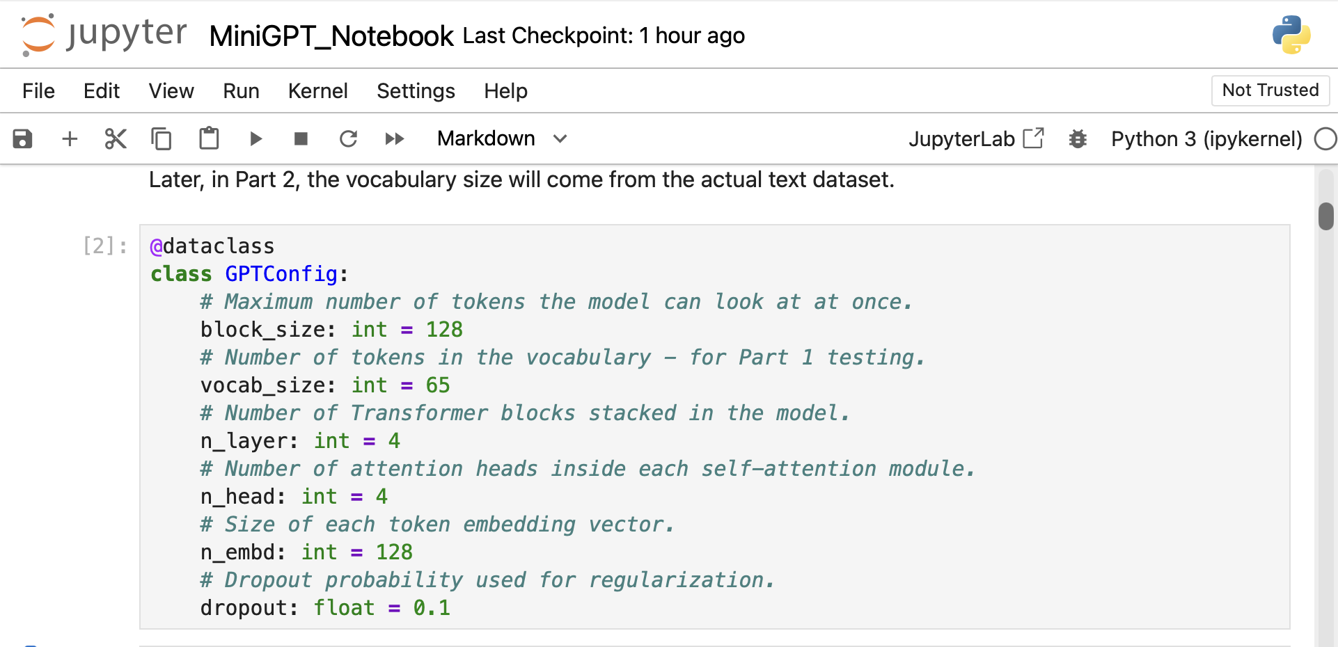
I ran the 1.1 cell, which defines GPTConfig with the small model's defaults
The cell prints nothing when I run it. It only defines a class. No model exists and no memory is used until section 1.6 creates a configuration and builds a model from it.
The @dataclass decorator reads the annotated fields and writes the class's __init__ (plus a readable __repr__ and an == comparison) for me. That lets me create a configuration with the defaults, GPTConfig(), or override only the fields I want to change, such as GPTConfig(n_layer=6, n_embd=384). The class has no behaviour of its own. It is a named bundle of numbers that every part of the model reads from.
Each field controls one dimension of the model:
block_sizeis the context length: the maximum number of letters the model can see at once. It sets the size of the position-embedding table and of the causal mask, so the model cannot look further back than this.vocab_sizeis the number of distinct tokens. It sets the number of rows in the token-embedding table and the number of scores the output layer produces at each position. The default of 65 is a placeholder for testing the model before any data is loaded. It happens to match the 65 letters in Tiny Shakespeare, and the later cells pass in the real value calculated from the text.n_layeris the number of Transformer blocks stacked on top of one another.n_headis the number of attention heads in each block. The attention code checks thatn_embddivides evenly byn_head, because each hidden state's query, key, and value are cut into one equal piece per head: 128 / 4 gives 32 numbers per head.n_embdis the width of the model: the length of every embedding, and so of the vector that represents each position at every layer. Most of the parameter count grows with the square of this number.dropoutrandomly switches off some numbers during training, to make it harder for the model to memorise its text. When running,model.eval()turns it off.
It helps me to picture the data inside the model as a spreadsheet, with one row per position and one column per number in its hidden state:
 Scroll sideways, or tap the diagram to open it full size
block_size limits the rows (letters), n_embd sets the columns (numbers per letter), and n_layer is how many times the sheet is processed
My exhibit uses exactly these defaults, so GPTConfig() with no arguments builds a machine of the right shape for my trained numbers.
The code, in the order the machine runs
Each layer above showed its own lines of the notebook. This section is the map: where each piece lives in the code, and the writing loop that runs the whole model. The notebook defines its classes bottom-up: attention in 1.2, the MLP in 1.3, one block in 1.4, and the whole model in 1.5. The machine runs the other way round, in the order of the five steps. Two kinds of line do nothing while the machine is writing, so I leave them out: the dropout lines, which model.eval() switches off, and the training-only lines that work out the loss, the score that training tries to lower, explained in the next post.
Every piece in this post is either a fixed set of numbers stored on the model, or a variable that the code works out while it runs:
| In this post | In the code | Fixed or changing? | Shape for goo |
|---|---|---|---|
| the letter IDs | idx | changing | 1 × 3 |
| all 65 token embeddings | model.token_embedding.weight; row 45 is the g embedding | fixed | 65 × 128 |
| all 128 position embeddings | model.position_embedding.weight | fixed | 128 × 128 |
| the hidden states | x, inside MiniGPT.forward | changing | 1 × 3 × 128 |
| block 1's query weights | model.blocks[0].attn.query.weight and .bias | fixed | 128 × 128 and 128 |
| the queries, keys, and values | q, k, and v, inside CausalSelfAttention.forward | changing | 1 × 3 × 128 each |
| the shares of attention | attn | changing | 1 × 4 × 3 × 3 |
all 65 rows of lm_head | model.lm_head.weight; row 42 is the d row | fixed | 65 × 128 |
lm_head's biases | model.lm_head.bias | fixed | 65 |
| the scores | logits | changing | 1 × 3 × 65 |
| the chances | probs | changing | 1 × 65 |
The first number in most shapes is the batch size, B: how many texts the code handles at once. While training, it handles 32 snippets at a time. While writing, it handles just one, so B is 1. The second number is T, the number of letters in the row, which is 3 for goo.
The writing loop: generate_text
Writing starts in generate_text, which the notebook defines in section 3.12. Each time round its loop, it chooses one new letter:
PYTHON
1# keep only the last 128 letter IDs
2idx_cond = idx[:, -model.config.block_size:]
3# steps 1 to 4: run the whole model
4logits, _ = model(idx_cond)
idx holds the letter IDs written so far: [[45, 53, 53]] for goo. The first line is the context limit from How much can it see at once?: it keeps only the last block_size letters, because there are no position embeddings beyond that. The second line runs the whole model, which calls MiniGPT.forward.
Run my model yourself
Everything in this post can be reproduced with three things: the notebook's model code (sections 1.1 to 1.5), my trained numbers, and the 65 letters in the right order. The quickest way is my follow-along workbook, which has all three and reproduces every number in this post, step by step, from the letter IDs to the GGUF file: open it in Colab, or download it. The steps below do the same in the notebook itself. I ran these steps myself, from scratch, in a fresh copy of the notebook, and the pictures below are that run. Any CPU is fast enough.
First, run the notebook's code cells from the top down to the end of section 1.5. That defines GPTConfig and the four classes, but builds nothing yet. Then add four new cells.
Cell 1: download my trained numbers. This is the checkpoint from Where every fixed number lives: all 826,433 fixed numbers, under the names the notebook's code expects, in a 3.4 MB file. It is the same model that runs in the live demo.
PYTHON
1import urllib.request
2
3# my trained numbers: the checkpoint, 3.4 MB
4urllib.request.urlretrieve("https://haddley.github.io/minigpt-demo/exhibit.pt", "exhibit.pt")

I ran the cell in a fresh folder, and it downloaded the 3.4 MB checkpoint. The line it prints just confirms the file name
Cell 2: build the machine, load the numbers, and run goo.
PYTHON
1# the 65 letters, in order: the position of each one is its ID
2chars = list("\n !$&',-.3:;?ABCDEFGHIJKLMNOPQRSTUVWXYZabcdefghijklmnopqrstuvwxyz")
3stoi = {ch: i for i, ch in enumerate(chars)}
4
5# build the machine, and load my numbers into it
6model = MiniGPT(GPTConfig())
7model.load_state_dict(torch.load("exhibit.pt", map_location="cpu"))
8model.eval()                 # running, not training: dropout off
9model.requires_grad_(False)  # and no records for training
10
11# steps 1 to 4 for goo
12idx = torch.tensor([[stoi[ch] for ch in "goo"]])
13logits, _ = model(idx)
14probs = torch.softmax(logits[0, -1], dim=-1)
15for p, i in zip(*torch.topk(probs, 4)):
16    print(repr(chars[i]), f"{p.item():.1%}")
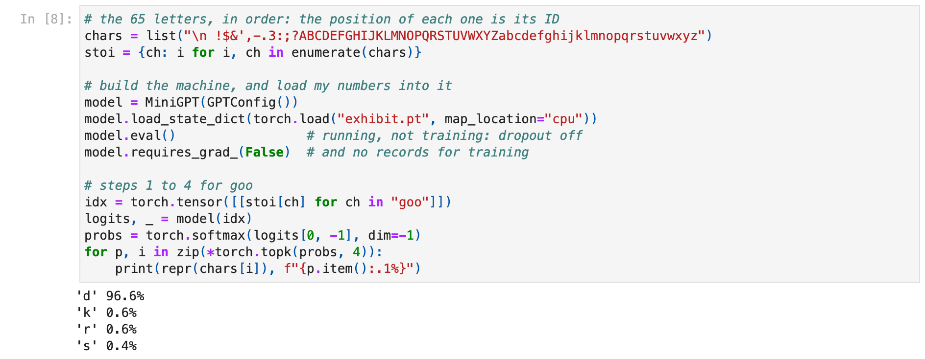
I ran the cell, and got exactly the chances from step 4: d 96.6%
Each piece has a job:
charsis the vocabulary: every letter that appears in Tiny Shakespeare, sorted into the computer's standard order, which puts the new line first, then the space and punctuation, then the capitals, then the lowercase letters. The order matters, because a letter's ID is simply its place in this list, and my token embeddings and rows oflm_headare stored in that order. The notebook builds the same list from the text withsorted(list(set(text)))in section 2.2.GPTConfig()with no arguments has exactly my model's settings: 4 blocks, 4 heads, 128 numbers per vector, 128 positions, and 65 letters. The checkpoint only fits a machine of that shape.load_state_dictcopies my numbers into the machine, replacing the random ones it was built with.model.eval()switches off dropout, which is only for training, andmodel.requires_grad_(False)tells PyTorch not to keep the extra records that training needs.
Cell 3: look at the parameters. Each line prints the start of one fixed table from this post:
PYTHON
1print(stoi["g"], stoi["o"], stoi["d"])                  # the letter IDs from step 1
2print(model.token_embedding.weight[stoi["g"]][:4])      # the g token embedding
3print(model.position_embedding.weight[0][:4])           # the position 1 embedding
4print(model.lm_head.weight[stoi["d"]][:4])              # the d row of lm_head
5print(model.blocks[0].attn.query.weight.shape)          # block 1's query weights
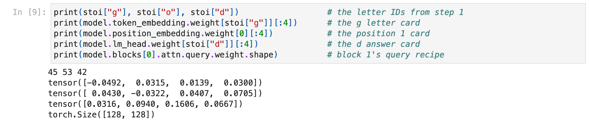
The IDs from step 1, then the first four numbers of the g token embedding, the position 1 embedding, and the d row of lm_head, and the size of block 1's query weights
Cell 4: write, by spinning the wheel. This loop is a cut-down generate_text, with a temperature of 0.8 and no trimming. The first line fixes the random spins, so that with the same version of PyTorch you get exactly the text I got; remove it, and every run writes something different.
PYTHON
1torch.manual_seed(1)   # remove this line for a different spin each time
2idx = torch.tensor([[stoi[ch] for ch in "ROMEO:\n"]])
3for _ in range(200):
4    logits, _ = model(idx[:, -model.config.block_size:])
5    probs = torch.softmax(logits[0, -1] / 0.8, dim=-1)
6    next_id = torch.multinomial(probs, num_samples=1)
7    idx = torch.cat([idx, next_id.view(1, 1)], dim=1)
8print("".join(chars[i] for i in idx[0].tolist()))
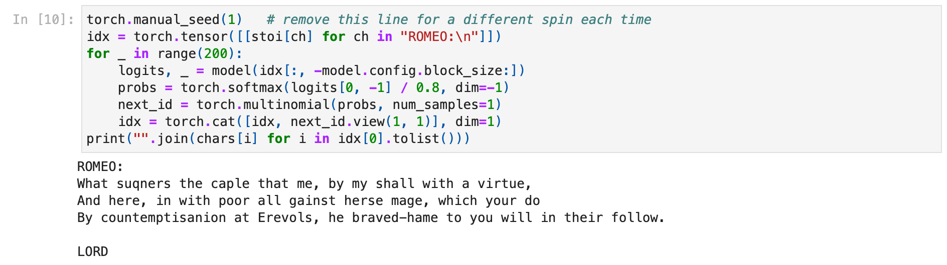
200 letters, chosen one spin at a time, after ROMEO: and a new line
Run it without Python: a GGUF file for llama.cpp
llama.cpp is the program behind many of the tools that run language models on a laptop, and it reads models from a single GGUF file: the fixed numbers, plus a note of which design to run and what the tokens are. I exported my model as one, exhibit.gguf, 3.3 MB, and checked it against PyTorch. On a Mac, these two commands install llama.cpp and make it write:
BASH
1brew install llama.cpp
2llama-completion -m exhibit.gguf -p $'ROMEO:\n' -n 120 --temp 0.8 --top-k 0 --top-p 1.0 --min-p 0
One run of mine wrote:
CODE
1ROMEO:
2For a duch a signer house?
3
4YORK:
5No ress you taken that is curse.
6
7EXTER:
8Where the bring a pattity mish, ble look no g
llama.cpp has no MiniGPT of its own, but it does run GPT-2, and MiniGPT is built the same way: learned position embeddings, normalising before attention and before the MLP, biases everywhere, and a separate lm_head. So the export script relabels each set of numbers with the name llama.cpp expects for GPT-2, and makes two adjustments:
- Query, key, and value weights go into one grid. llama.cpp keeps the three tables stacked, one above the other, as a single 384 × 128 grid.
lm_head's biases move. llama.cpp's GPT-2 has no biases on itslm_head, but my model does. The final normalisation adds its own fixed numbers just beforelm_head, so I changed those instead, by exactly the amount that gives every letter the same score as before. Because the 65 rows oflm_headare all different from each other, there is exactly one way to do that, and the scores match to within a millionth.
The tokens are the 65 letters, written the way GPT-2 stores them: the space as Ġ and the new line as Ċ, so goo still becomes 45, 53, 53. llama.cpp also insists on an "end of text" token, which my model never learned. Left to itself, llama.cpp picked token 11, which is ;, and stopped writing at the first semicolon, so I nominated $ instead: it appears exactly once in all of Tiny Shakespeare.
I compared all 65 chances from llama.cpp with PyTorch's, for four different texts:
| Text ends with | Top letter | PyTorch | llama.cpp | Biggest difference among all 65 letters |
|---|---|---|---|---|
goo | d | 96.63% | 96.63% | 0.001 points |
good m | y | 40.81% | 40.80% | 0.013 points |
my kingdom for a hors | e | 76.57% | 76.61% | 0.035 points |
hear me spea | k | 97.97% | 97.96% | 0.001 points |
The tiny differences come from the MLP's bend, GELU: llama.cpp uses a fast approximation of the curve that the notebook calculates exactly. And like PyTorch, llama.cpp stops at 128 letters, because there are no more position embeddings.
Try it yourself
- The paper: MiniGPT: Rebuilding GPT from First Principles (arXiv:2605.17398)
- Play with a real one: Transformer Explainer runs GPT-2 in your browser and shows attention and the chances for your own text, and LLM Visualization walks through a small GPT in 3D, one calculation at a time
- Build one step by step: MicroGPT Visualized starts from counting pairs of letters and adds one idea at a time
- My follow-along workbook: open it in Colab. It runs my trained model and reproduces every number in this post
- The notebook: github.com/jibin10/MiniGPT : open
MiniGPT_Notebook.ipynbin Colab, or clone it and run it locally, then follow Run my model yourself to load my trained model. Any CPU will do