MiniGPT (Part 4)
Neil Haddley • October 5, 2026
The same machine on a faster engine: rebuilding MiniGPT in Apple's MLX, what one shared pool of memory, lazy calculation, and compiling the training step buy, and a fair race against PyTorch on the same Mac, with a follow-along notebook
Part 3 settled the pieces: my own 8,192-piece tokeniser matched GPT-2's on TinyStories, at under half the size. This post keeps that machine exactly as it is, the same blocks, the same embeddings, the same stories, and changes only the engine underneath it: the library that does the arithmetic. Parts 1 to 3 used PyTorch. This post rebuilds the machine in MLX, Apple's library for machine learning on its own chips, and races the two on the same Mac.
I have used MLX before, in MLX 1, but only to fine-tune a model someone else had released. This post writes the machine itself in MLX: the layers, the training step, and the gradient.
The code is in part4-mlx/, with a follow-along notebook, minigpt_follow_along_4.ipynb. MLX only runs on Apple Silicon, so the notebook is for running on a Mac, not in Colab.
| This post's machine | |
|---|---|
| What changed | the engine |
| Text | TinyStories |
| Pieces | my 8,192 |
| Blocks | 6, each attention (6 heads) then an MLP |
| Vector size | 384 |
| Positions | 256, position embeddings |
| Engine | MLX |
| Size | 13.9 million numbers |
| Score | 0.689 bits per byte |
The big picture, in plain English
Same machine, different engine
A library like PyTorch or MLX is the engine under the machine. The machine says what to calculate: look up the token embeddings, run attention, run the MLP, score the rows of lm_head. The engine decides how: where the numbers are kept, when each calculation runs, and how the calculations are packed together for the chip. Change the engine, and the same calculations can run faster, or in less memory, without the answers changing.
MLX was designed around three things about Apple's chips, and each one is a chance to save work.
One shared pool of memory
Most computers keep two separate stores of memory: one for the main processor, and one on the graphics chip, the GPU, which does the heavy arithmetic. Every batch of training text has to be copied from one to the other before the GPU can use it. PyTorch is built for that kind of computer, so its code is full of instructions to move things across:
PYTHON
1x = x.to(device) # copy the batch to the GPU
Apple's chips have one pool of memory that the processor and the GPU share. MLX is built around that, so there is nothing to copy and no .to(device) anywhere: the training batch goes straight into an MLX array, and the GPU reads it where it is. On my 64 GB Mac Studio, all 64 GB is available to the machine.
Calculating only when asked
PyTorch calculates each line the moment it runs. MLX does not. When a line says "multiply these" or "add those", MLX writes the step down and waits. Nothing is calculated until something actually needs a result: printing a number, or an explicit mx.eval.
That sounds like a delay, but it gives MLX the whole list of steps before it starts, so it can see which ones can be done together, and which ones are never needed at all. The name for it is lazy evaluation.
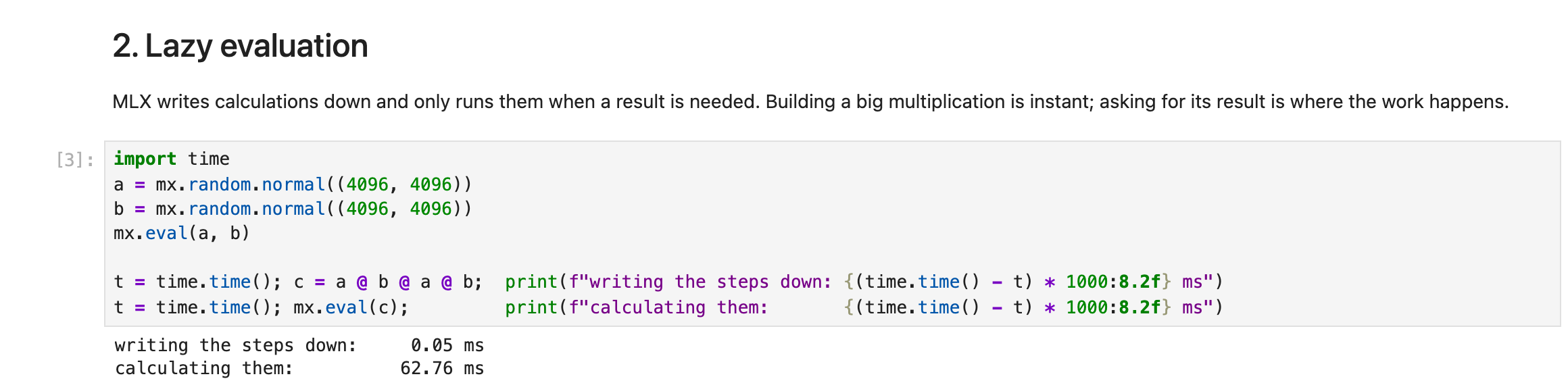
The follow-along notebook in Jupyter on my Mac, timing lazy evaluation: writing a big multiplication down took 0.05 milliseconds, and the work, 63 milliseconds, happened at mx.eval
 Scroll sideways, or tap the diagram to open it full size
The same four lines on each engine. PyTorch sends the GPU a job for every line; MLX writes lines 1 and 2 down and runs them together at mx.eval
Packing the whole training step into one
Because MLX writes the steps down first, it can do something bigger: take one whole training step (the trip forward, the trip back that finds every parameter's slope, capping the slopes if they are unusually big, and turning the parameters) and compile it, which packs it into a single combined job for the GPU. That saves the GPU from starting and stopping between thousands of small jobs. In MLX it is one line, mx.compile, and it turns out to be where almost all of the speed comes from.
The race
I raced three engines on the same machine, the same batch of 32 snippets of 256 tokens, on the same Mac Studio. bench.py times 200 training steps of each, after 20 warm-up steps, each in its own fresh program so that the memory figures stay clean.
| Engine | Tokens per second | Most memory used |
|---|---|---|
| PyTorch, on the Mac's GPU | 48,426 | 4.60 GB |
| MLX, not compiled | 45,106 | 3.72 GB |
| MLX, compiled | 56,136 | 3.89 GB |
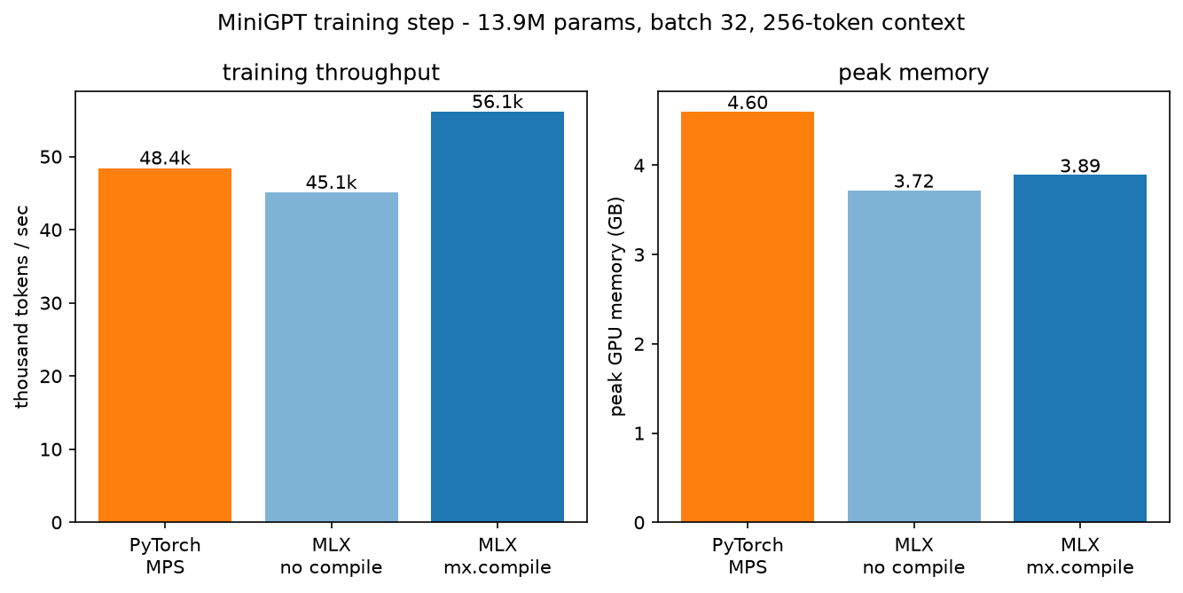
The same three runs as bars: speed on the left, memory on the right
Two things stand out:
- Compiling is where the speed is. Without
mx.compile, MLX is slightly slower than PyTorch. With it, MLX is about a quarter faster than itself, and 16% faster than PyTorch. When the notebook ran the same race again later, compiled MLX came out 20% faster, so the honest range from my runs is 16 to 20%. - MLX uses less memory either way: 3.7 to 3.9 GB against PyTorch's 4.6 GB, about 15 to 20% less for exactly the same machine. Later in this series, when a much bigger teacher model has to share the same pool, that headroom matters.
Same answers?
A faster engine is no use if it changes the answers. The two versions do not start from exactly the same random numbers, because the two libraries draw their starting parameters differently, so their training curves cannot lie exactly on top of each other. But they should end up in the same place, and they do: after 3,000 steps, the MLX machine scores 0.689 bits per byte on the test stories, and the PyTorch machine from Part 3 scores 0.697. That gap is about the size of the luck between two random starts of the same machine: in Part 5, three random starts of one design scored up to 0.007 apart.
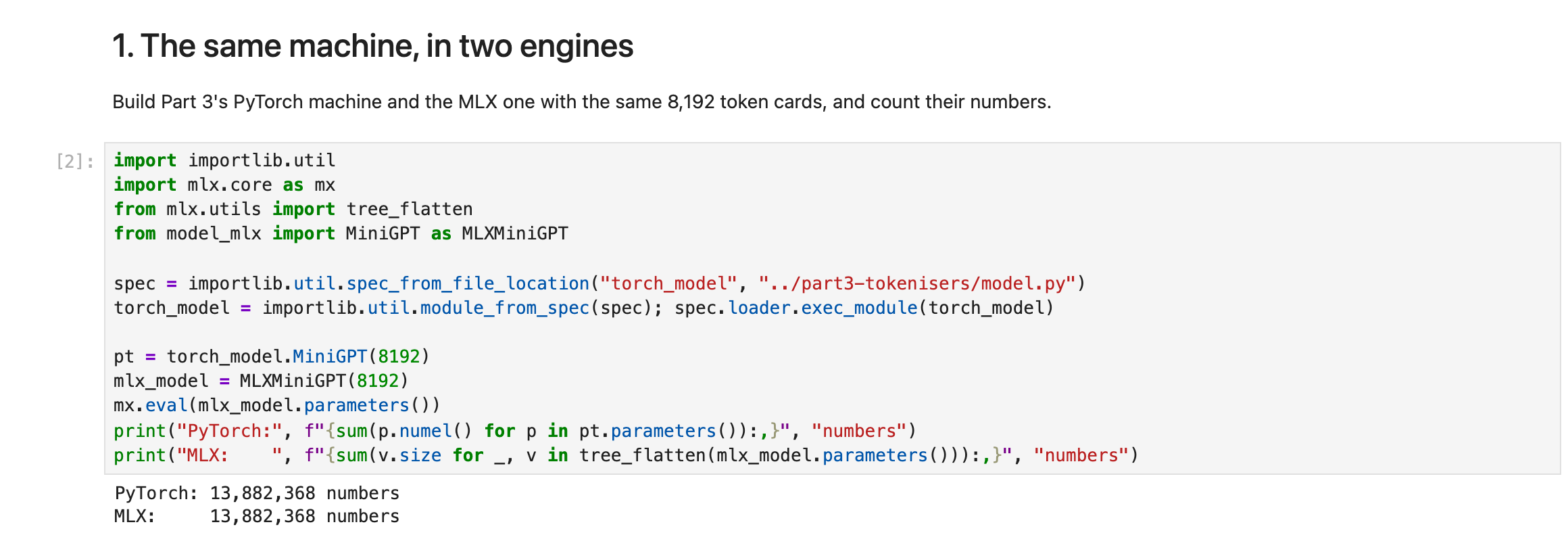
The notebook built the same machine in both engines, and counted exactly the same 13,882,368 numbers in each
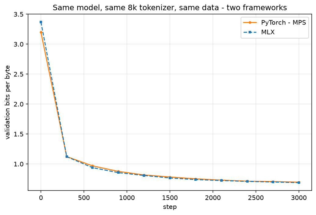
Bits per byte on the test stories while training, PyTorch against MLX
And they write the same kind of story:
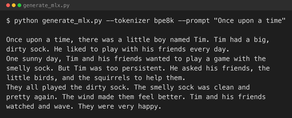
The MLX machine continuing "Once upon a time"
Tim has a dirty sock, the sock stays the subject of the story, and the story has a beginning, a middle, and an end. It makes the same kinds of slips as the PyTorch machine, such as "watched and wave", and longer samples drift in the same way. The port made the same machine, not just a machine with a similar score.
The jargon decoder
The terms for the whole series are collected in one table, the series glossary.
| What I called it | What the experts call it |
|---|---|
| the engine | the framework |
| one shared pool of memory | unified memory |
| writing calculations down and running them later | lazy evaluation |
| packing a whole step into one job | compiling, with mx.compile |
| the slopes of every parameter, all together | the gradient |
| capping the slopes if they are unusually big | gradient clipping |
| copying a batch to the GPU | a host-to-device transfer |
The code, in the order it runs
The code is in part4-mlx/. It reuses the stories and tokenisers that Part 3's scripts prepare, so data.py reads them from part3-tokenisers/data/.
The machine: model_mlx.py
The machine is Part 3's, line for line, with three small differences. First, attention is one built-in call, which does the query, key, and value matching, the earlier-positions-only rule, and the shares, all in one fused job:
PYTHON
1out = mx.fast.scaled_dot_product_attention(q, k, v, scale=self.scale, mask="causal")
The hand-written version in Part 1 is still the one to read to understand attention; this is the one to run.
Second, the token embeddings double as the rows of lm_head without any bookkeeping, because there is no separate answer layer at all: the last hidden states are simply scored against the token embeddings.
PYTHON
1def __call__(self, idx):
2    x = self.tok_emb(idx) + self.pos_emb(mx.arange(idx.shape[1]))
3    for block in self.blocks:
4        x = block(x)
5    x = self.ln_f(x)
6    return x @ self.tok_emb.weight.T   # the token embeddings are the output rows
Third, there is no .to(device), anywhere.
The training step: train_mlx.py
In PyTorch, the trip back that finds every parameter's slope happens as a side effect of loss.backward(), as Part 2 showed. In MLX it is a function: nn.value_and_grad takes the machine and its surprise-score function, and gives back a new function that returns the score and every parameter's slope, as an ordinary value. The whole step is then compiled:
PYTHON
1loss_and_grad = nn.value_and_grad(model, MiniGPT.loss)
2state = [model.state, opt.state]
3
4@partial(mx.compile, inputs=state, outputs=state)
5def train_step(x, y):
6    loss, grads = loss_and_grad(model, x, y)
7    grads, _ = optim.clip_grad_norm(grads, 1.0)
8    opt.update(model, grads)
9    return loss
inputs=state, outputs=state tells MLX that the compiled step is allowed to change the machine's parameters and the optimiser's memory. Then the training loop makes each step happen:
PYTHON
1for step in range(args.iters + 1):
2    xb, yb = batch(train_ids, args.block_size, args.batch_size, rng)
3    loss = train_step(mx.array(xb), mx.array(yb))
4    mx.eval(state)          # the step is calculated here
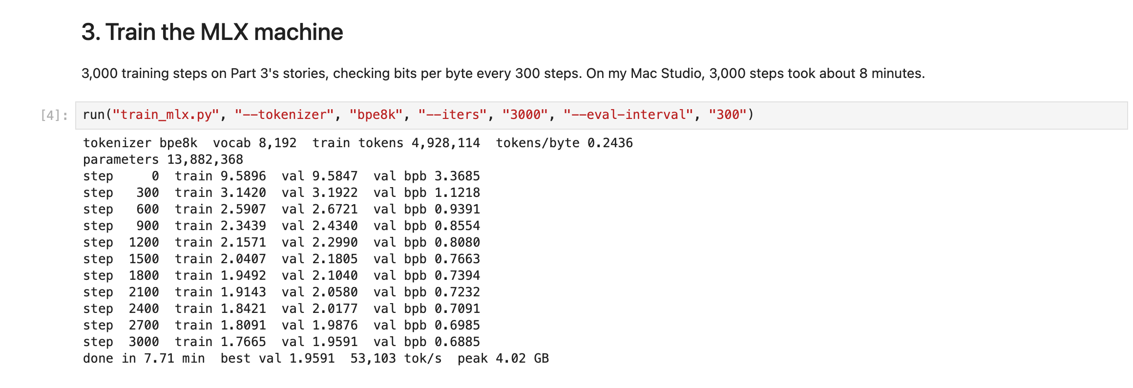
The MLX training run in the notebook: 3,000 steps, the same 8k tokeniser and stories as Part 3, finishing at 0.6885 bits per byte
The race: bench.py
bench.py --framework torch, --framework mlx-nocompile, and --framework mlx each time 200 training steps of the same machine, after 20 warm-up steps, and report tokens per second and the most memory used. Each runs as its own program, so one cannot inherit another's memory.

The three races
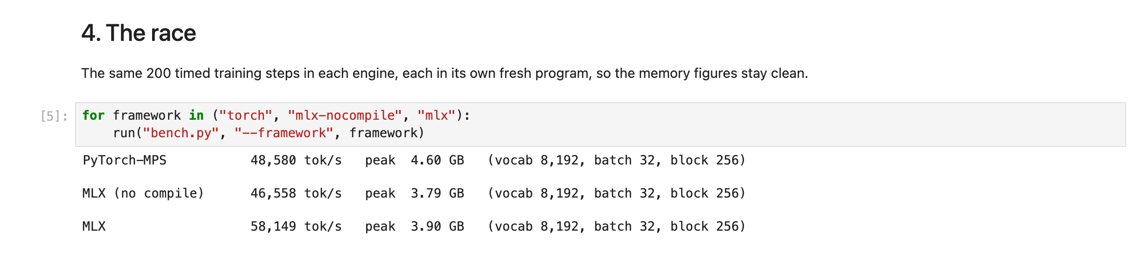
The same race, run again later in the notebook: this time compiled MLX was 20% faster than PyTorch
Writing: generate_mlx.py
PYTHON
1idx = mx.array([tok.encode("Once upon a time")])
2for _ in range(300):
3    logits = model(idx[:, -model.block_size:])[:, -1, :]
4    idx = mx.concatenate([idx, sample(logits, temperature=0.8, top_k=200)], axis=1)
5print(tok.decode(idx[0].tolist()))
The same loop as every part so far: score the last hidden state against the rows of lm_head, spin the wheel, and put the new token on the end.
Try it yourself
- The follow-along notebook:
part4-mlx/minigpt_follow_along_4.ipynb. Open it in Jupyter on a Mac with Apple Silicon. It prepares the stories, checks that the MLX machine has the same 13.9 million numbers as Part 3's, trains it, runs the race, and writes. It is saved with the outputs from my own run, so you can read every result on GitHub without a Mac.
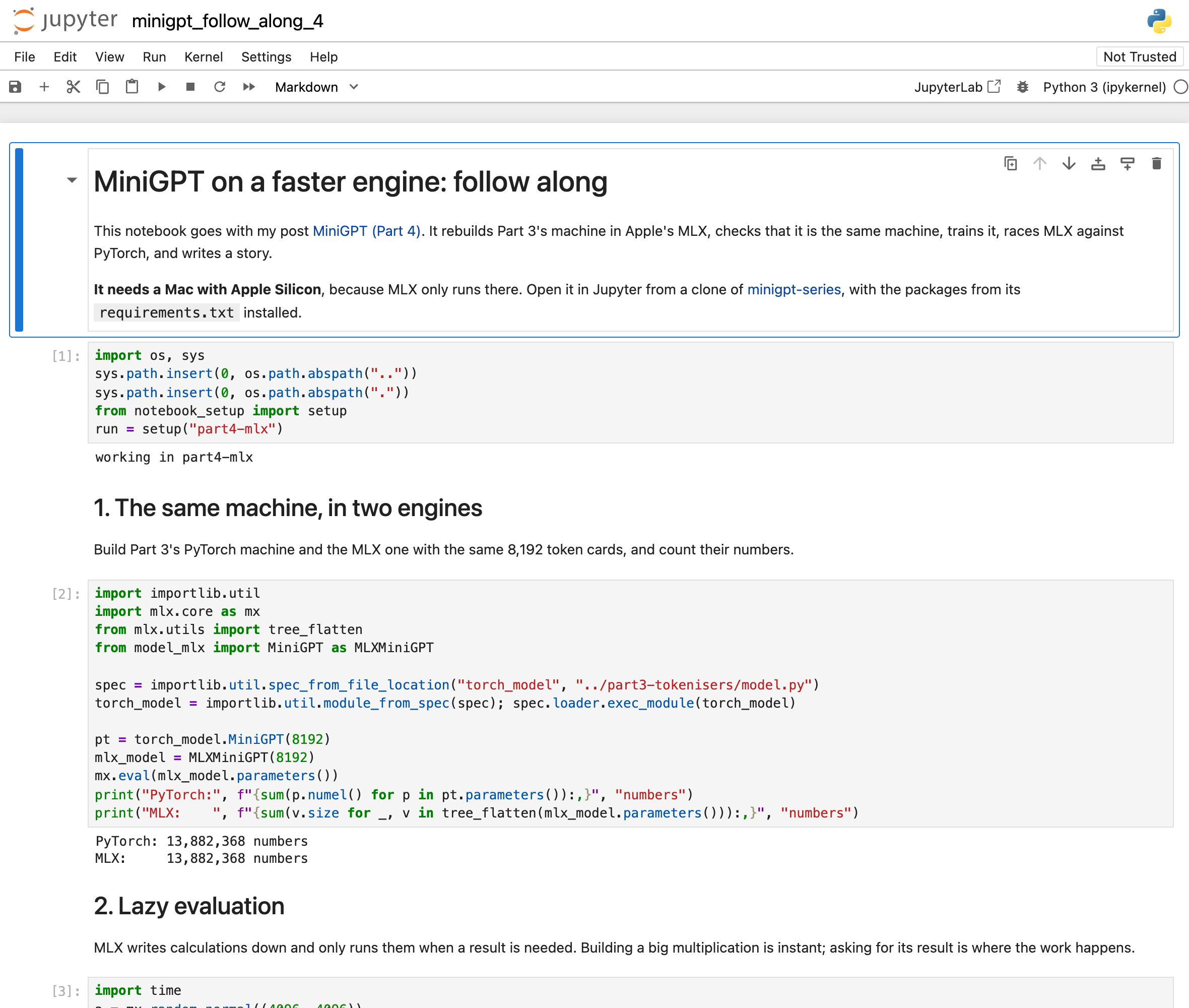
The notebook open in Jupyter on my Mac, with the outputs saved from my run
- On the command line:
BASH
1git clone https://github.com/Haddley/minigpt-series.git
2cd minigpt-series
3python3 -m venv .venv && source .venv/bin/activate && pip install -r requirements.txt
4cd part3-tokenisers && python prepare_data.py && python tokenizers_setup.py && cd ..
5cd part4-mlx
6python train_mlx.py --tokenizer bpe8k --iters 3000 --eval-interval 300
7python bench.py --framework torch
8python bench.py --framework mlx-nocompile
9python bench.py --framework mlx
10python generate_mlx.py --prompt "Once upon a time"