MiniGPT (Part 7)
Neil Haddley • October 5, 2026
Reading a longer row in the same memory: why attention's cost grows with the square of the row, how a sliding window caps it, why writing the window as a mask saves nothing, and a secret-word test of what a long row is for, and of how far a window really reaches, with a follow-along notebook
Part 1 warned that a longer row of positions is expensive, mostly because of attention. This post measures exactly how expensive, on the modern machine from Part 5, and then fixes it with the trick Mistral's models use: let each hidden state look back only over a fixed window of recent positions.
The code is in part7-sliding-window/, with a follow-along notebook for a Mac, minigpt_follow_along_7.ipynb.
| This post's machine | |
|---|---|
| What changed | a longer row, read through a sliding window |
| Text | TinyStories |
| Pieces | my 8,192 |
| Blocks | 6 of Llama's design, from Part 5 |
| Vector size | 384 |
| Positions | 1,024, each hidden state looking back at most 256; no position embeddings |
| Engine | MLX |
| Size | 12.6 million numbers |
| Score | 0.6727 bits per byte |
The big picture, in plain English
Why a longer row costs so much
In attention, every hidden state matches its query against the key of every earlier position, and itself. So the number of matches grows much faster than the row.
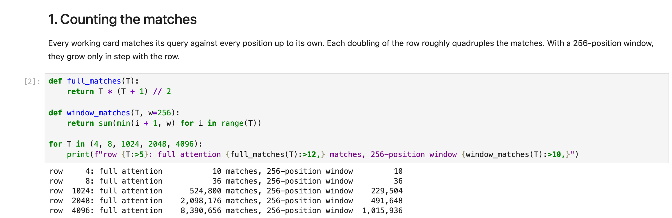
The follow-along notebook in Jupyter on my Mac, counting the matches for one head. Full attention's count quadruples with each doubling of the row; the window's only doubles
Every one of those matches is a number the machine has to hold while it trains, in every head of every block. Double the row and you need about four times the memory for attention. On a machine with one fixed pool of memory, that is the wall you hit first.
A sliding window
The fix is to let each hidden state look back only over a fixed window, here the last 256 positions, however long the row is. Then each hidden state makes at most 256 matches, and the total grows only in step with the row: twice the row, twice the matches.
In principle, through the blocks. In block 1, a hidden state gathers information from up to 256 positions back. In block 2, it looks at hidden states that have already gathered from their own windows, so it could reach up to about 512 back, and so on. With 6 blocks, information could travel about 1,500 positions, one window per block, much as Part 1's four blocks let each hidden state reach further back than the one before. But could is not does: the secret-word test below found that my machine never learned to do it.
Writing the window as a mask saves nothing
The obvious way to build the window is the way the earlier-positions rule is built: a grid of "allowed" and "not allowed", here also blocking anything more than 256 positions back. It gives exactly the right behaviour. But it saves no memory at all: the machine still works out every match in the full row-by-row grid, and only then throws most of them away.
To actually save memory, the machine must never build the full grid. So the row is cut into chunks of 256 positions, and each chunk only looks at itself and the chunk before it. That covers every hidden state's window, and the biggest grid ever built is 256 by 512, however long the row.
 Scroll sideways, or tap the diagram to open it full size
The same window, built two ways, for a row of 16 positions. The mask builds the whole grid and throws most of it away; the chunks never build the squares that would be thrown away
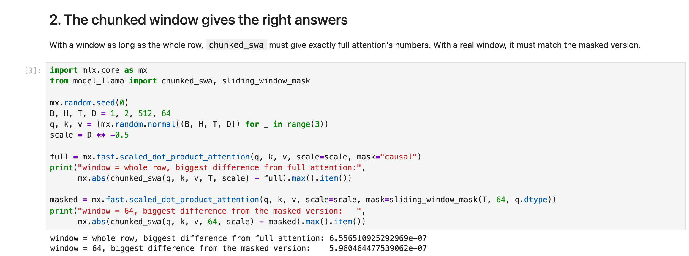
The notebook checked that the chunks give the right answers: against full attention when the window covers the whole row, and against the mask when it does not. Both differences are rounding
The memory race
mem_sweep.py trains the 12.6-million-number modern machine for a few steps at each row length, three ways, and records the most memory each used:
| Row length | Full attention | Window, as a mask | Window, in chunks |
|---|---|---|---|
| 512 | 2.55 GB | 2.60 GB | 2.67 GB |
| 2,048 | 11.5 GB | 11.5 GB | 7.7 GB |
| 4,096 | 35.5 GB | 35.4 GB | 15.1 GB |
| 8,192 | not run: about 120 GB | not run | 30.0 GB |
| 16,384 | not run: about 450 GB | not run | 59.4 GB |
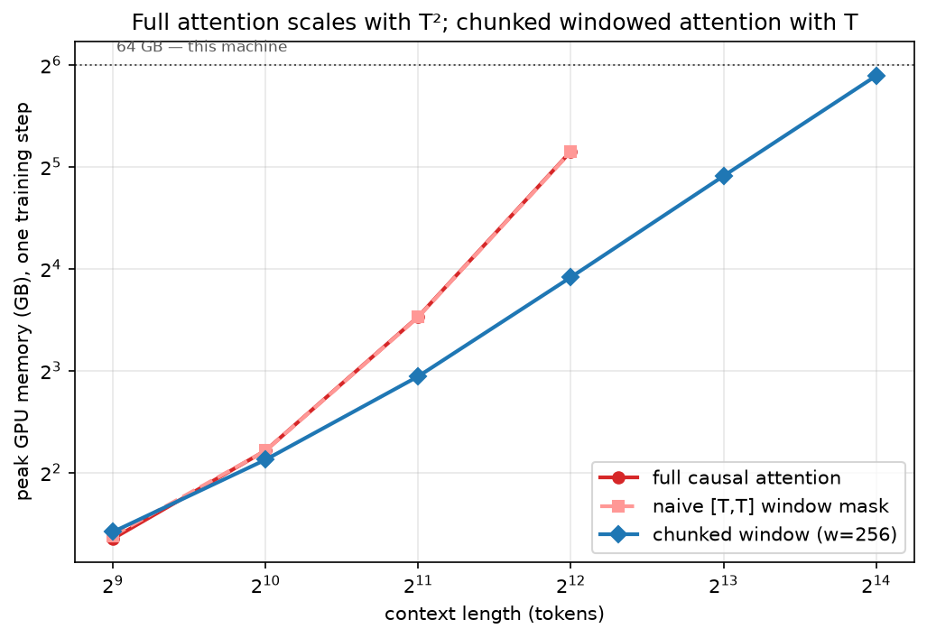
Most memory used, against row length. Full attention and the masked window are the same line; the chunked window climbs much more gently
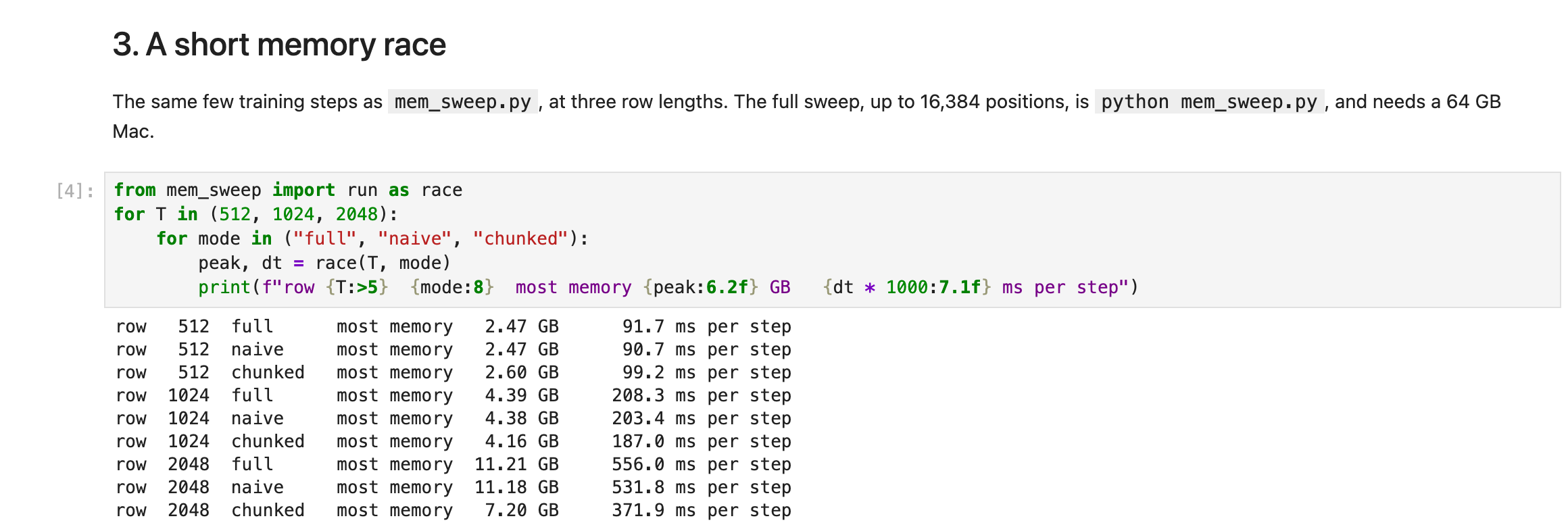
The notebook's shorter race, up to 2,048 positions. Already at 2,048, the chunks use 7.2 GB against full attention's 11.2 GB
- The mask column matches full attention at every length, exactly as the last section predicted.
- At short rows, everything is close. Most of the memory then goes on the MLPs and on scoring against 8,192 rows of
lm_head, and both of those grow only in step with the row. Attention takes over at about 2,048 positions. - At 4,096, full attention needs 35.5 GB, more than half the Mac, and 1.9 seconds a step. The chunked window needs 15.1 GB and 0.8 seconds. At 8,192, full attention would need more memory than the Mac has. The chunked window reaches 16,384 positions in 59.4 GB.
Does the windowed machine still learn?
A window is only useful if the machine still works. I trained the modern machine with a row of 1,024 positions, four times the length used in Parts 3 to 6, once with full attention and once with a 256-position window, for 1,500 steps each:
| Attention | Bits per byte | Minutes | Most memory used |
|---|---|---|---|
| full | 0.6805 | 9.8 | 8.39 GB |
| 256-position window | 0.6727 | 9.0 | 7.66 GB |
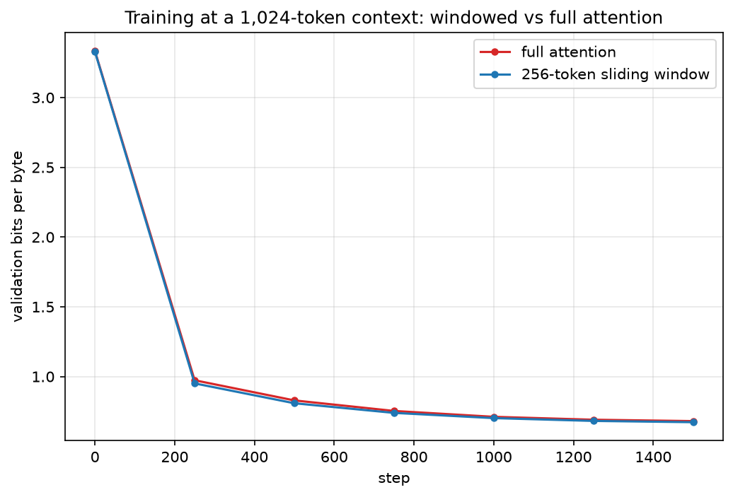
Bits per byte at a 1,024-position row. The windowed machine is not behind
The windowed machine came out slightly ahead, but only by 0.008, about the size of the luck between two random starts (see Part 5), so the two are level. It also trained faster and in less memory. And its 0.6727 is inside the band of Part 5's 256-position machine (0.672 to 0.678, over three random starts): on these stories, a longer row did not help at all, because most stories are only a few hundred tokens long, so there is nothing further back worth seeing. TinyStories is the wrong text to show what a long row is for, so the next section builds a test that is not. The point here is the memory: on these stories, the windowed machine learns just as well, while its attention cost stays flat as the row grows.
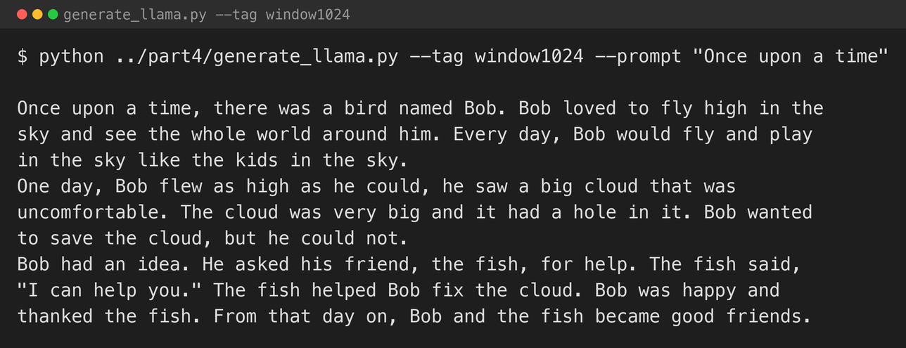
The windowed machine, with a 1,024-position row, continuing "Once upon a time"
A bird named Bob, a fish that helps him, and "they became good friends": the same shape of story as every machine in this series. The window cost it nothing you can see.
What is a long row for? The secret word
TinyStories cannot show what a long row is for, so I built a test that can. Each test row hides a secret near its start, such as " Lily's secret word is apple.", then carries on with ordinary stories, and ends by asking for it again: " Lily's secret word is". There are 8 names and 24 words, so a machine that cannot see the secret can only guess, right 1 time in 24. Half of each training batch was rows like these, with the secret anywhere from 20 to 1,000 pieces back; the other half was ordinary stories. I trained three machines on exactly this mix, 1,500 steps each, and then asked each one for the word from five distances, 400 times at each:
| Machine | 100 back | 200 back | 400 back | 700 back | 970 back |
|---|---|---|---|---|---|
| 256-position row | 100% | 100% | 4.2% | 4.2% | 4.2% |
| 1,024-position row, full attention | 100% | 100% | 100% | 100% | 100% |
| 1,024-position row, 256-position window | 100% | 100% | 3.8% | 3.8% | 3.8% |
| the same window machine, trained 4 times longer | 100% | 100% | 4.5% | 4.5% | 4.5% |
 Scroll sideways, or tap the diagram to open it full size
The same results as a picture. Inside 256 pieces, all three machines find the word every time; beyond it, only full attention does
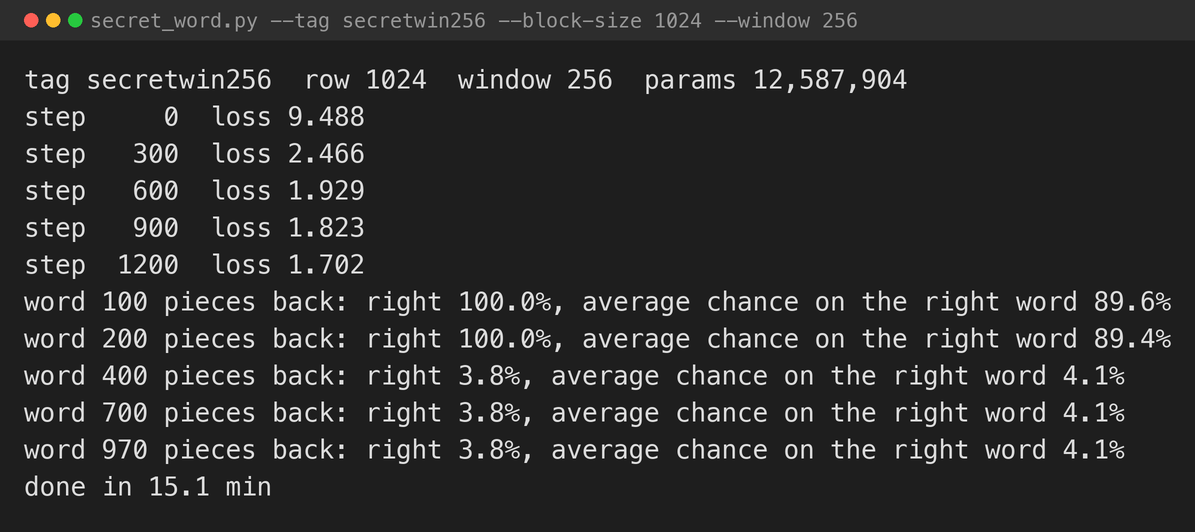
The window machine's own run: it learned the trick close up, and guessed beyond its window
- All three learned the trick. Whenever the secret was inside what they could see, all three got it right every time.
- The 256-position row cannot see past its row. Beyond 256 pieces, the secret has fallen off the front, and it can only guess.
- Full attention can. With 1,024 positions, it found the word 970 pieces back every time. This is what a long row is for.
- The window did not reach past its window. It behaved exactly like the 256-position row. Through six blocks, the word could have hopped 256 positions at a time to the end, but in 1,500 steps of training the machine never learned to pass it along. Training it four times longer, 6,000 steps, only made it surer of the word close up (96% of the chance on the right word, up from 89%); beyond its window, it still guessed.
My reading of why: to pass the word along, some hidden state in the middle of an unrelated story would have to pick the secret up in one block and hold it for a later block to collect, and no part of that chain is rewarded until the whole chain works. Whatever the reason, the lesson is the same: the reach that the blocks allow in principle is not reach the machine has learned. It is one reason why many models that use windows, such as Google's Gemma 2, also keep some blocks with full attention.
The jargon decoder
The terms for the whole series are collected in one table, the series glossary.
| What I called it | What the experts call it |
|---|---|
| the length of the row | the context length, or sequence length |
| looking back only a fixed number of positions | sliding-window attention |
| the grid of allowed matches | the attention mask |
| growing with the square of the row | quadratic, or O(T²), cost |
| growing in step with the row | linear, or O(T × W), cost |
| how far information could travel through the blocks | the receptive field |
| some blocks with a window, and some with full attention | interleaved, or local and global, attention |
The code, in the order it runs
The windowed attention lives in Part 5's model_llama.py, behind a window setting, and part7-sliding-window/ measures it.
The mask that saves nothing: sliding_window_mask
PYTHON
1i = mx.arange(T)[:, None]
2j = mx.arange(T)[None, :]
3keep = (j <= i) & (i - j < w)          # earlier positions only, and at most w back
4return mx.where(keep, mx.array(0.0, dtype), mx.array(-mx.inf, dtype))
This builds the full T-by-T grid, and the attention call still works out every match before the mask removes most of them.
The chunks that do save: chunked_swa
PYTHON
1qc = q.reshape(B, H, nc, w, D)                                            # queries, in chunks of w
2kc = mx.stack([kpad[:, :, i * w:i * w + 2 * w] for i in range(nc)], axis=2)  # each chunk's keys, plus the chunk before
3vc = mx.stack([vpad[:, :, i * w:i * w + 2 * w] for i in range(nc)], axis=2)
4scores = (qc @ kc.transpose(0, 1, 2, 4, 3)) * scale                       # never bigger than w by 2w
5scores = mx.where(mask[None, None], scores, -mx.inf)
6out = mx.softmax(scores, axis=-1) @ vc
The biggest grid is [batch, heads, chunks, w, 2w], which grows in step with the row. With a window as long as the row, it gives exactly the same numbers as full attention.
Choosing between them: Attention in model_llama.py
PYTHON
1if self.window <= 0:
2    out = mx.fast.scaled_dot_product_attention(q, k, v, scale=self.scale, mask="causal")
3elif self.naive_window:
4    m = sliding_window_mask(T, self.window, x.dtype)
5    out = mx.fast.scaled_dot_product_attention(q, k, v, scale=self.scale, mask=m)
6else:
7    out = chunked_swa(q, k, v, self.window, self.scale)   # after sharing out the key and value heads
The secret word: secret_word.py
secret_word.py builds each secret row from Part 3's stories, mixes them half and half with ordinary stories, trains one machine, and then asks for the word from 100 to 970 pieces back. A 256-position machine sees only the last 256 pieces of each row:
PYTHON
1secret = tok.encode(f" {name}'s secret word is {word}.")
2question = tok.encode(f" {name}'s secret word is") + tok.encode(f" {word}")
3row = np.concatenate([ids[s:s + before], secret, ids[s + before:s + before + gap], question])
run_secret.sh trains the three machines: --block-size 256, --block-size 1024, and --block-size 1024 --window 256, and then the window machine again with --iters 6000.
The race: mem_sweep.py
For each row length from 512 to 16,384, and each of the three ways, mem_sweep.py builds the machine, trains it for 5 steps on random tokens, and records the most memory used and the time per step. It skips full attention and the mask past 4,096 positions, where they would run the Mac out of memory.
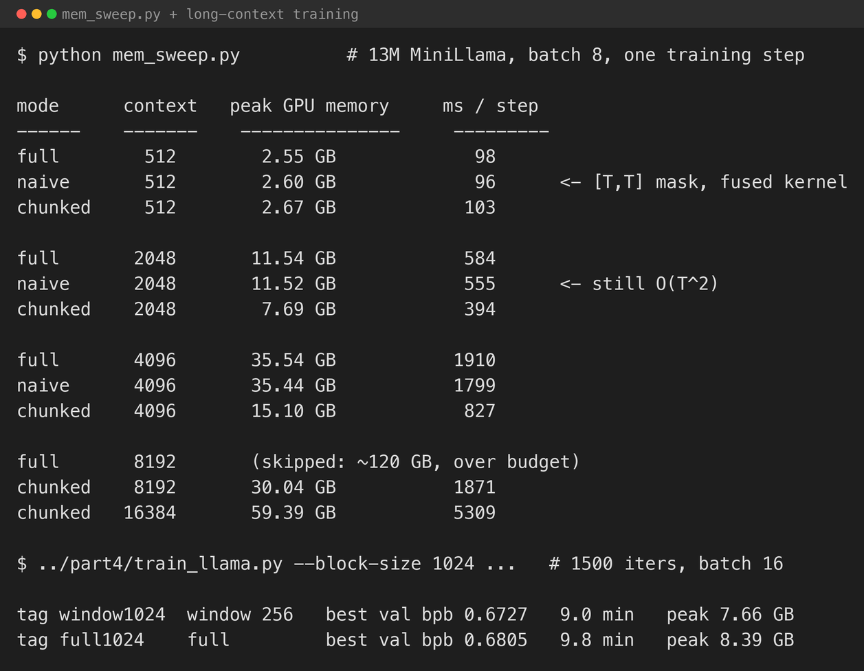
The sweep's own output, and the two training runs
The series
Seven parts, from a character-level GPT in a borrowed notebook to a modern small model in MLX:
- Running it: a trained MiniGPT taken apart while it writes.
- Growing it: training the same machine from random numbers.
- Pieces, not letters: three tokenisers, scored fairly in bits per byte.
- A faster engine: the same machine in Apple's MLX.
- The modern block: Llama's four changes, one at a time. Only RoPE mattered.
- Learning from a teacher: distillation, and why the most helpful teacher was not the best storyteller.
- Reading further: sliding-window attention.
Every machine here is tiny, and none of them is good. That was the point. The tokeniser, the training loop, the engine, and the tricks, distillation, shared keys and values, and windowed attention, are all things you can build and run in an afternoon on one Mac. What separates them from the models I use every day is scale: more text, more numbers, and more computing, applied to substantially the same design.
The series glossary
Every idea in this series in plain words, next to the name the experts use, and the part whose jargon decoder it first appears in. Each term is explained in that part.
| In plain words | What the experts call it | First in |
|---|---|---|
| the guessing game | next-token prediction, or language modelling | Part 1 |
| a letter: any of the 65 symbols, even the space and the comma | a character | Part 1 |
| the thing being guessed: a letter here, a word or piece of a word in big models | a token | Part 1 |
| the 65 letters | the vocabulary | Part 1 |
| the chances for each possible next letter | a probability distribution, produced by a softmax | Part 1 |
| a letter's row of 128 learned numbers | its token embedding (token_embedding): a vector | Part 1 |
| a position's row of 128 learned numbers | the position embedding (position_embedding) | Part 1 |
| a token embedding plus its position embedding, before block 1 | the input embedding | Part 1 |
| the number of positions: how many letters it can see at once | the context length, or context window (block_size) | Part 1 |
| "only look at earlier positions" | the causal mask | Part 1 |
| what attention matches and collects | the query, the key, and the value vectors | Part 1 |
| the three tables of weights that make them | the query, key, and value projections (self.query, self.key, self.value) | Part 1 |
| keeping the keys and values instead of remaking them | the KV cache | Part 1 |
| add, never replace | the residual connection | Part 1 |
| the hidden states, as every block adds to them | the residual stream | Part 1 |
| a position's vector after a block | a hidden state | Part 1 |
| normalising a hidden state before attention and before the MLP | layer normalisation, or LayerNorm | Part 1 |
| every fixed number that training set | the parameters, or weights | Part 1 |
| spinning the wheel of chances | sampling | Part 1 |
| keeping the biggest k slices | top-k sampling | Part 1 |
| keeping the biggest slices until they add up to p | top-p, or nucleus, sampling | Part 1 |
| the 65 rows that score each letter that could come next | the language-model head (lm_head), or output layer | Part 1 |
| the scores, before softmax | the logits | Part 1 |
| a request the model writes for a program to carry out | a tool call, or function call | Part 1 |
| the program around the model | the harness | Part 1 |
| a harness letting the model act by itself for many steps | an agent | Part 1 |
| working out what the trained parameters mean | interpretability | Part 1 |
| learning from the text itself, with no people marking answers | self-supervised learning, or pre-training | Part 2 |
| people writing example conversations for the machine to copy | supervised fine-tuning (SFT) | Part 2 |
| people comparing answers, to train a judge | the reward model | Part 2 |
| practising against the judge | reinforcement learning from human feedback (RLHF), often using a method called PPO | Part 2 |
| letting another model do some of the comparing | reinforcement learning from AI feedback (RLAIF) | Part 2 |
| letting an existing model write the examples, or teach its chances | distillation | Part 2 |
| the surprise score | the loss (cross-entropy loss) | Part 2 |
| "as unsure as choosing between N letters" | perplexity | Part 2 |
| working out which way to turn every parameter | backpropagation | Part 2 |
| the 32 snippets for one step | a batch (batch size 32) | Part 2 |
| the slopes of all 826,433 parameters, together | the gradient | Part 2 |
| nudging every number a little in its direction | an optimiser step (here, with AdamW) | Part 2 |
| how far each nudge goes | the learning rate | Part 2 |
| AdamW's running average of recent slopes | momentum | Part 2 |
| shrinking every number very slightly on every step | weight decay | Part 2 |
| the locked-away exam text | the validation set | Part 2 |
| memorising the textbook | overfitting | Part 2 |
| keeping the best copy | checkpoint selection | Part 2 |
| walking downhill on the surprise-score landscape | gradient descent | Part 2 |
| the program that cuts text into pieces | the tokeniser | Part 3 |
| a piece's row of learned numbers, a word or part of a word as well as a letter | its token embedding | Part 3 |
| gluing the most common pair | a BPE merge | Part 3 |
using the token embeddings as the rows of lm_head too | weight tying | Part 3 |
| halvings of surprise for each byte of text | bits per byte | Part 3 |
| surprise per token | the loss, or cross-entropy | Part 3 |
| the engine | the framework | Part 4 |
| one shared pool of memory | unified memory | Part 4 |
| writing calculations down and running them later | lazy evaluation | Part 4 |
| packing a whole step into one job | compiling, with mx.compile | Part 4 |
| capping the slopes if they are unusually big | gradient clipping | Part 4 |
| copying a batch to the GPU | a host-to-device transfer | Part 4 |
| the simpler normalise | RMSNorm (root mean square normalisation) | Part 5 |
| the 2017 normalise | LayerNorm | Part 5 |
| turning queries and keys by position | rotary position embeddings, or RoPE | Part 5 |
| the MLP with a gate | SwiGLU | Part 5 |
| sharing keys and values between heads | grouped-query attention, or GQA | Part 5 |
| a query, key, and value for every head | multi-head attention, or MHA | Part 5 |
| turning one change off at a time | an ablation study | Part 5 |
| copying a teacher's whole wheel | logit distillation, or knowledge distillation | Part 6 |
| learning only from the right answer | training on a one-hot target, or hard labels | Part 6 |
| the teacher's wheel | soft targets | Part 6 |
| how different two wheels are | the KL divergence (Kullback–Leibler divergence) | Part 6 |
the raw scores against the rows of lm_head | the logits | Part 6 |
| the softening setting | the distillation temperature | Part 6 |
| a stronger teacher whose wheels the student cannot reach | the capacity gap | Part 6 |
| the length of the row | the context length, or sequence length | Part 7 |
| looking back only a fixed number of positions | sliding-window attention | Part 7 |
| the grid of allowed matches | the attention mask | Part 7 |
| growing with the square of the row | quadratic, or O(T²), cost | Part 7 |
| growing in step with the row | linear, or O(T × W), cost | Part 7 |
| how far information could travel through the blocks | the receptive field | Part 7 |
| some blocks with a window, and some with full attention | interleaved, or local and global, attention | Part 7 |
Try it yourself
- The follow-along notebook:
part7-sliding-window/minigpt_follow_along_7.ipynb, for Jupyter on a Mac with Apple Silicon. It counts the matches, checks that the chunked window gives full attention's numbers when the window covers the whole row, runs a short memory race, and shows the secret-word results. It is saved with the outputs from my own run, so you can read every result on GitHub without a Mac.
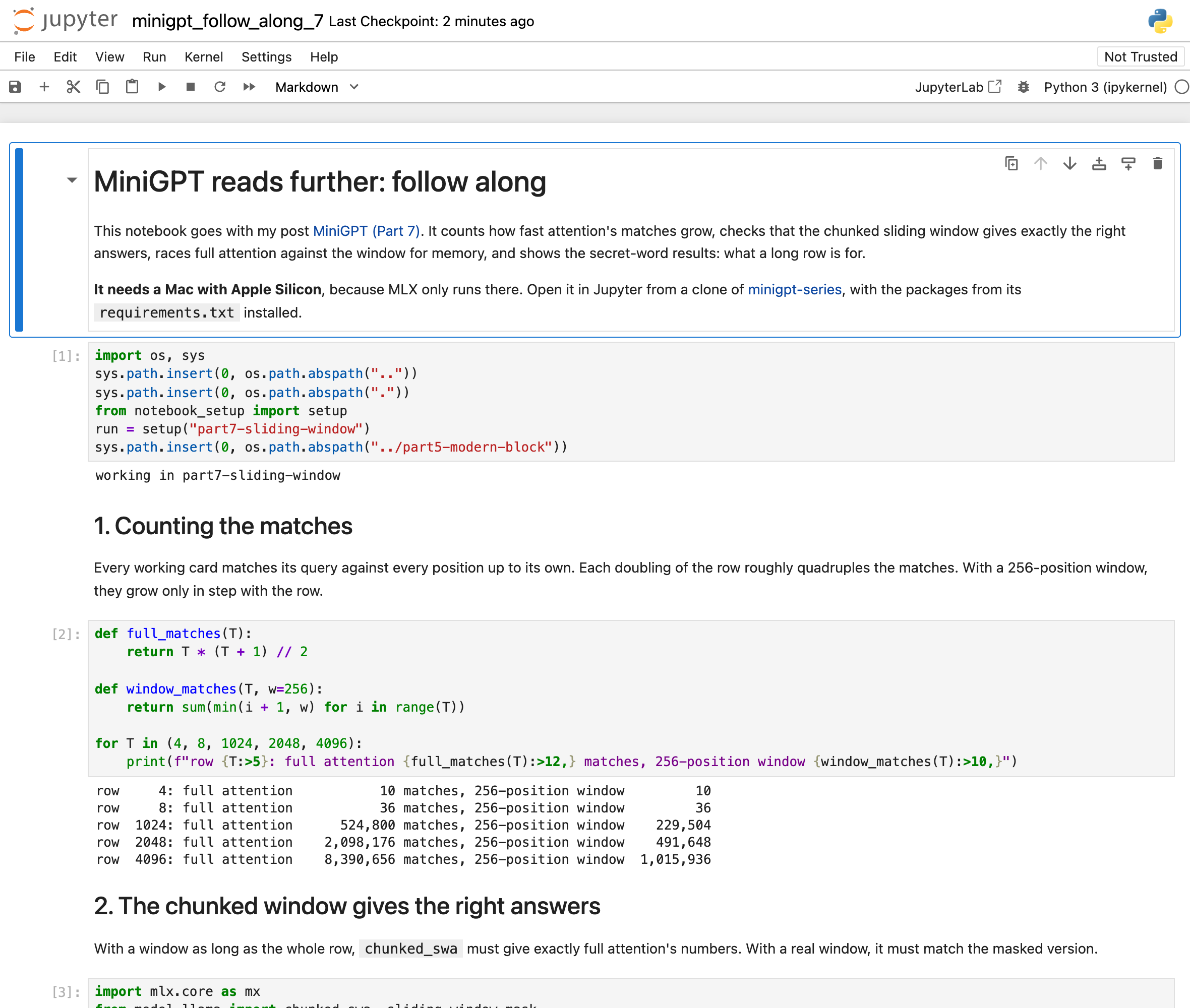
The notebook open in Jupyter on my Mac, with the outputs saved from my run
- On the command line, after Part 3's
prepare_data.pyandtokenizers_setup.py:
BASH
1cd minigpt-series/part7-sliding-window
2python mem_sweep.py
3python figures.py
4python ../part5-modern-block/train_llama.py --tag window1024 --block-size 1024 --window 256 --iters 1500
5python ../part5-modern-block/train_llama.py --tag full1024   --block-size 1024 --window 0   --iters 1500
6./run_secret.sh      # the secret-word test: three machines, then the window machine for longer; about 2 hours
MLX needs Apple Silicon.