Scikit-Learn (Part 11)

Neil Haddley • October 13, 2026

Training deep neural networks: why deep networks are hard to train, and the starting numbers, activation functions, batch normalization, optimizers, and dropout that make it work

AI Pythonmachine-learningneural-networkskerasoptimizersbatch-normalizationdropout

In Part 10, I trained a network with two hidden layers, and it worked. This chapter of the Hands-On Machine Learning book asks what goes wrong when a network gets deep, with tens or hundreds of layers. The example is deliberately extreme: a network with 100 hidden layers, learning to recognise clothing from Fashion MNIST, the same real pictures as before. The depth is the point. It is to show a failure, and the fixes.

With the right settings, the 100-layer network learned: 82.0% of validation pictures right after five passes. With ReLU, the usual choice from Part 10, the same network got only 69.9%. Smaller changes helped in the same way: a better way of nudging took one network from 83.7% to 87.9%, and reusing another network's layers took a tiny dataset of 200 pictures from 90.5% to 91.7%.

Key Points

The lesson: a deep network does not fail because it cannot represent the answer. It fails because the slopes, which backpropagation passes back through every layer, shrink or grow at each layer until the early layers barely learn. Almost every trick in this chapter is a way of keeping those slopes a sensible size, or of nudging more cleverly. Most are now the default in modern libraries, so the main thing is to know why they are there.

What I learned from it:

The numbers a network starts with matter. Starting them at the right size keeps the signal the same size as it passes through the layers.
The bend between layers matters. In my run, a bend called SELU (scaled exponential linear unit), with matching starting numbers, took the 100-layer network from 69.9% with ReLU to 82.0%.
How the nudging is done matters too: the same network scored 83.7% with plain gradient descent and 87.9% with AdamW, a smarter way of choosing each step. A different trick, rescaling each layer's inputs during training (batch normalization), let a network with only two hidden layers reach 86.7% after two passes.
Starting from a network that someone else has trained, and switching off a random few neurons during training (dropout), help when data is short or a network starts to memorise its training pictures.

The chapter also covers more bends than I used, more ways of nudging, and penalties for large numbers. I mention a few in the table below and do not go into the rest.

Quick Example

A network with 100 hidden layers of 100 neurons, built with the SELU activation function and the LeCun starting numbers that SELU needs:

PYTHON

1model = tf.keras.Sequential()
2model.add(tf.keras.layers.Flatten(input_shape=[28, 28]))
3for layer in range(100):
4    model.add(tf.keras.layers.Dense(100, activation="selu",
5                                    kernel_initializer="lecun_normal"))
6model.add(tf.keras.layers.Dense(10, activation="softmax"))
7model.compile(loss="sparse_categorical_crossentropy",
8              optimizer=tf.keras.optimizers.SGD(learning_rate=0.001),
9              metrics=["accuracy"])

Here is what the chapter's networks did when I ran the notebook. All of them learn Fashion MNIST from Part 10, and the percentages are of the 5,000 validation images unless I say otherwise:

Network	Result
100 layers, SELU, after 5 passes	82.0%
The same 100 layers with ReLU	69.9%
2 hidden layers, batch normalization, after 2 passes	86.7%
200 images, network trained from scratch (test)	90.5%
200 images, reusing another network's layers (test)	91.7%
3 hidden layers, plain SGD (stochastic gradient descent), after 10 passes	83.7%
The same network trained with AdamW	87.9%
The same network, with a step size that rises and then falls (the "1cycle" schedule), 25 passes	89.2%
2 hidden layers with dropout (test)	86.4%

So the 100-layer network does learn, but only just, and only with the right activation function. With ReLU, the same depth gets less than 70% after five passes.

Faster optimizers

The optimizer is the part of training that turns each slope into a nudge. I trained the same network, three hidden layers of 100 neurons, for 10 passes with each optimizer the chapter covers, all with a learning rate of 0.001:

Optimizer	Validation accuracy
SGD	83.7%
AdaGrad	84.1%
RMSProp	85.9%
Momentum	86.1%
Nesterov	86.4%
Adamax	87.2%
Adam	87.4%
Nadam	87.5%
AdamW	87.9%

Every optimizer after plain SGD keeps a running memory for each number. Momentum and Nesterov remember the average slope, so a number that keeps being pushed the same way speeds up. AdaGrad and RMSProp remember the average size of the slope, and give each number its own step size. Adam and its relatives keep both memories, and they did best in my run.

What training means here

This is still backpropagation, the same recipe as Part 10: start from random numbers, score the surprise on a batch, find every number's slope by working backwards, and nudge. Every trick in this chapter fits somewhere in that loop:

Trick	Where it fits in the loop
He and Glorot initialization	how the random starting numbers are chosen
ReLU, SELU, GELU, and the rest	the bends between layers, which decide whether slopes can get back
Batch normalization	extra layers that keep each layer's inputs a sensible size
Reusing pretrained layers	starting from numbers another network has already learned
Adam and AdamW	how each slope becomes a nudge
Learning rate schedules	how big the nudges are at each point in training
Dropout	switching neurons off at random, so that no neuron can rely on another

Batch normalization also shows that not every number in a network is nudged. Its layers add 4,736 numbers to the network: half of them are learned by backpropagation, and the other half, 2,368 running averages of the inputs, are simply updated as training goes. Keras counts them as "non-trainable".

My MiniGPT model uses several of these tricks. It starts its numbers small and random, trains with AdamW, normalizes inside every block with layer normalization, a close cousin of batch normalization, and trained with dropout. Its 826,433 numbers are nudged by the same loop as the networks in this chapter.

There are no Dumb Questions

Q: If backpropagation is the same in Part 10 and Part 11, what actually changed?

A: The network's arithmetic stayed the same; what changed is how well the slopes survive the trip back through the layers, and what the optimizer does with them. A slope that has shrunk to almost nothing gives almost no nudge, however many passes you make.

Q: Why does ReLU do worse than SELU in the 100-layer network, when ReLU is the usual choice?

A: SELU was designed so that, with the right starting numbers and scaled inputs, each layer's outputs keep roughly the same average and spread, even through 100 layers. ReLU has no such guarantee. Real deep networks usually add batch normalization or skip connections instead, and then ReLU works well.

Q: What are Swish and Mish?

A: They are two more activation functions, smooth bends like ReLU. Swish multiplies each input by its own sigmoid, the S-shaped curve that squashes any number to between 0 and 1. Big positive inputs pass through almost unchanged, big negative inputs are squashed towards zero, and in between there is a small dip below zero. Mish is a smoother cousin of Swish. Neither name is an acronym: Swish was found by an automated search, and Mish is named after its inventor, Diganta Misra. The notebook draws GELU, Swish, and Mish next to each other, below, and they look very alike.

Q: Does dropout make the network worse at its job?

A: During training, yes, a little, on purpose: 20% of the neurons are switched off at random on every step. When the network is used, every neuron is switched back on. My dropout network got 88.4% of the training images and 86.4% of the test images right, a small gap, which is what dropout is for.

Q: What is Monte Carlo (MC) dropout for?

A: It leaves dropout switched on when the network is used, and asks the same question 100 times. The answers vary, and the spread shows how sure the network is. For the first test image, the plain network said ankle boot with 80.9% confidence; the average of 100 dropout runs said 71.0% ankle boot and 22.3% sneaker, with a lot of disagreement between the runs. It is right, but less sure than it first claimed.

Running the notebook in Jupyter

The chapter is in the notebook that goes with the book, 11_training_deep_neural_networks.ipynb. I ran everything before the exercise solutions, which took about 9 minutes on my Mac Studio, and then looked through the results in JupyterLab.

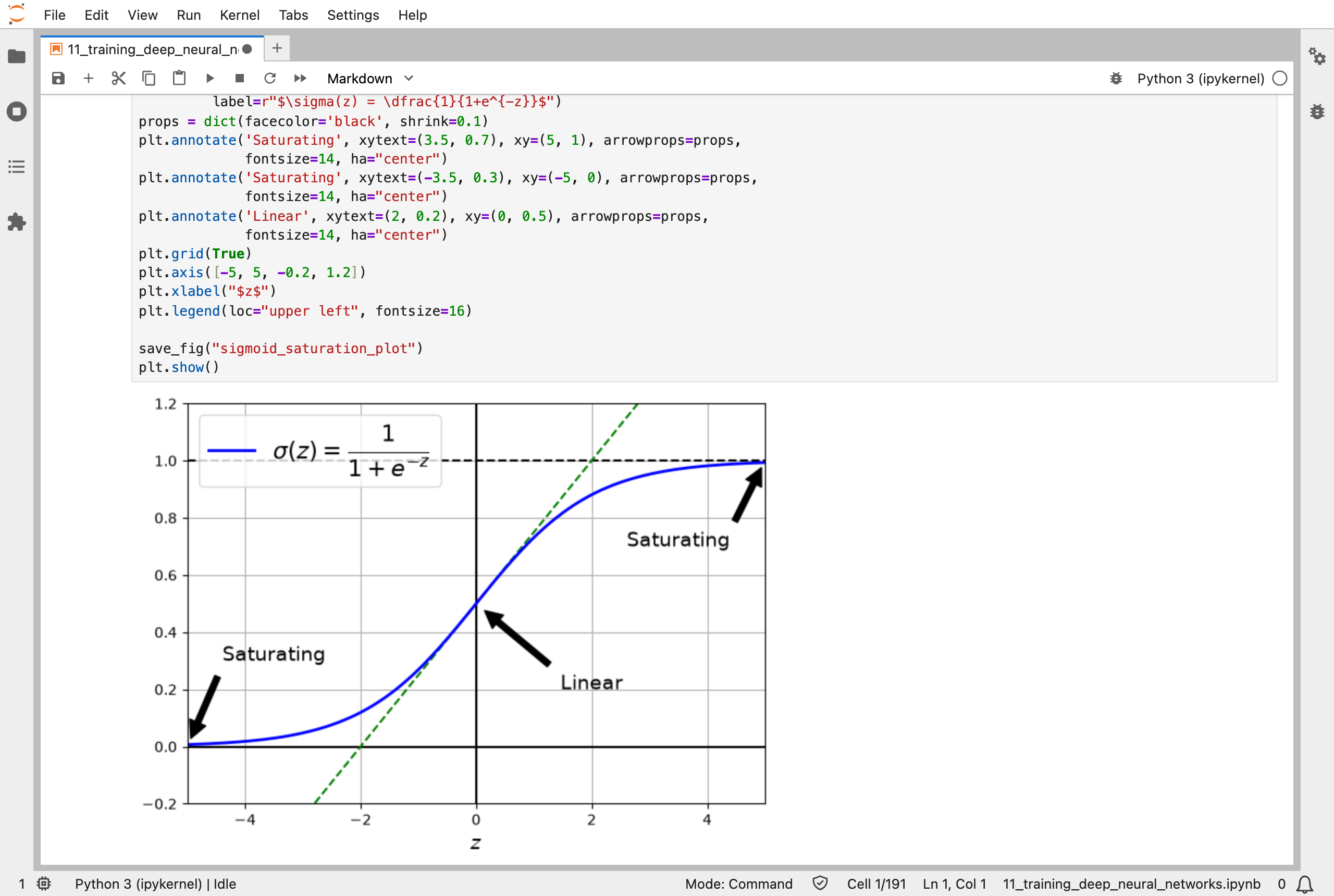
The sigmoid function goes flat at both ends: there its slope is almost zero, so the slopes passed back through it almost vanish

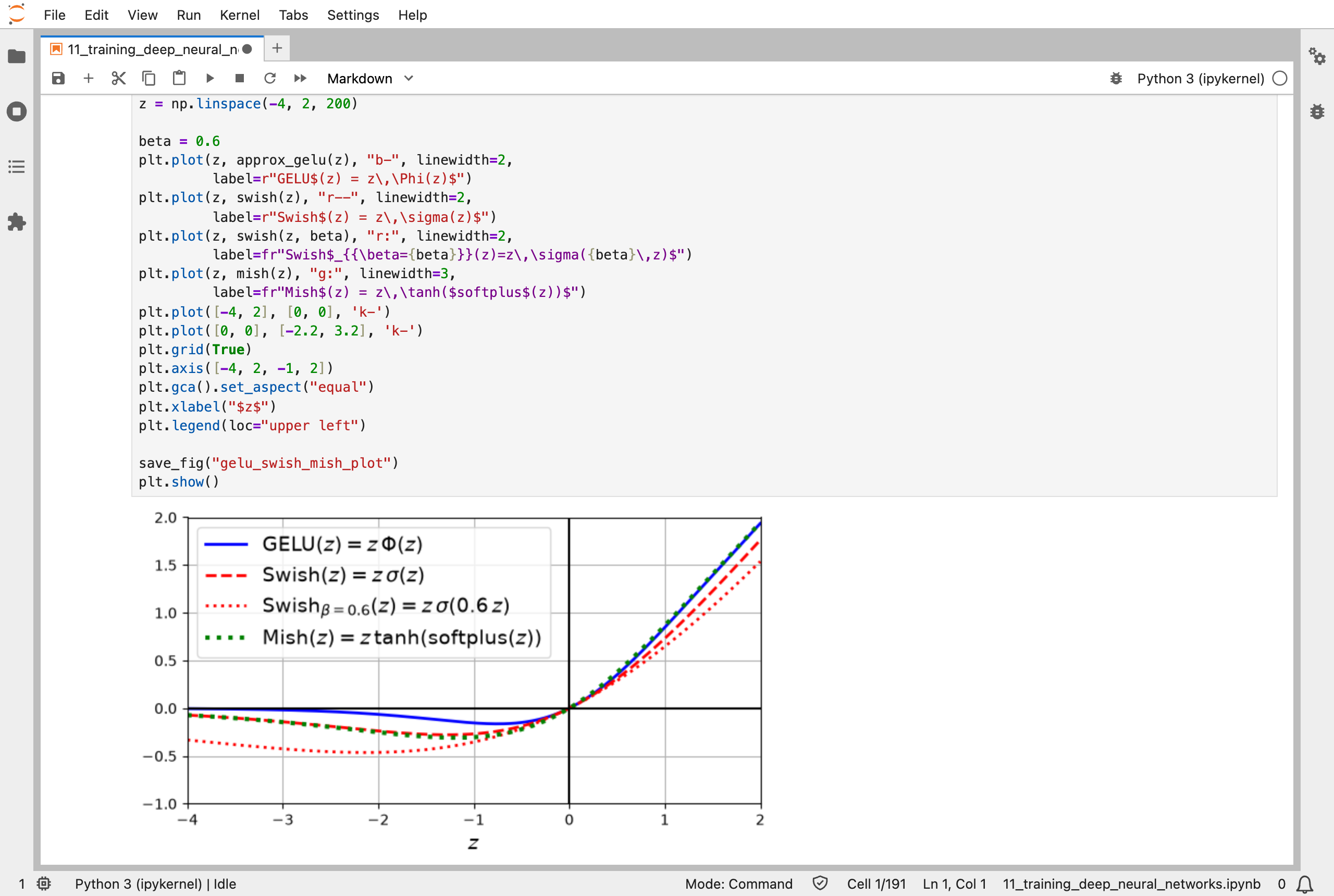
GELU, Swish, and Mish: smooth bends that, like ReLU, keep a slope for positive inputs, but dip a little below zero

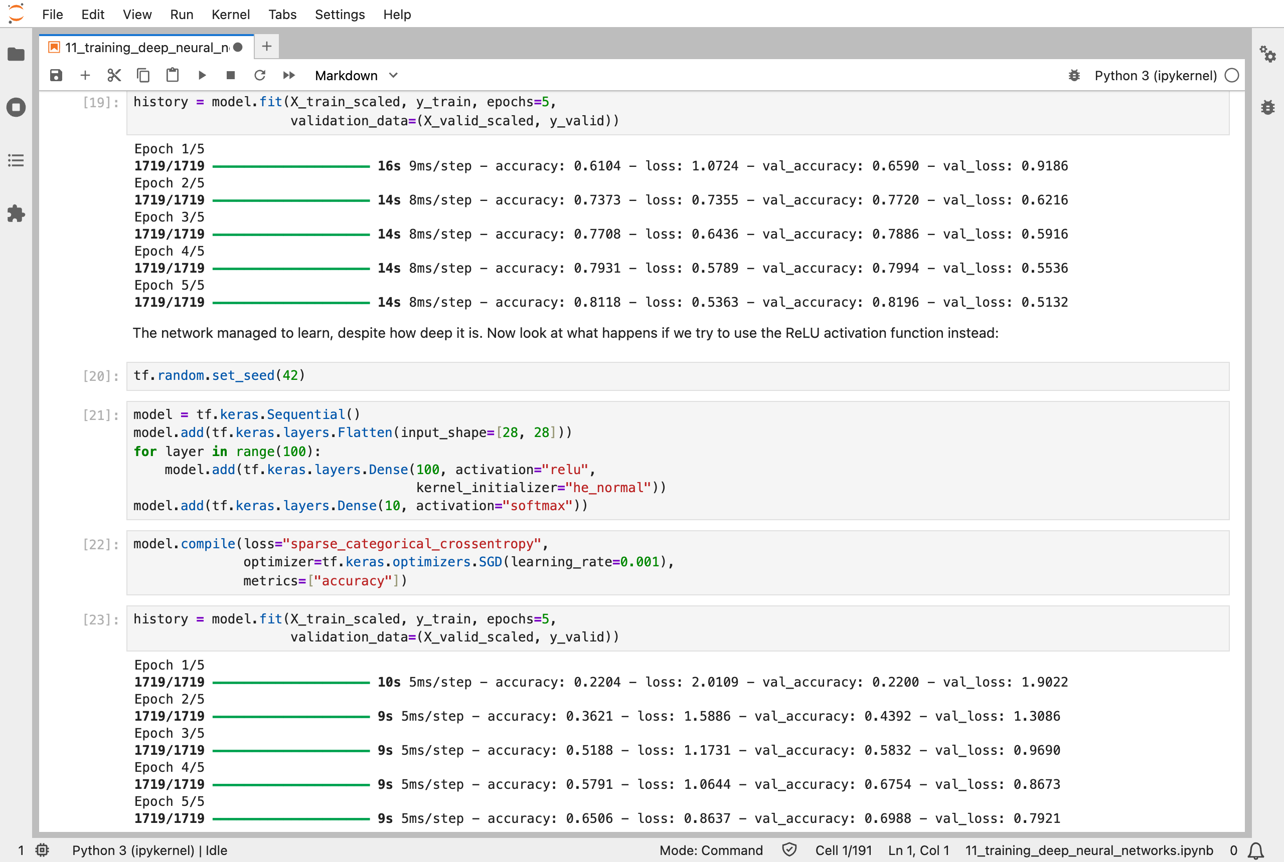
Two networks with 100 hidden layers: with SELU (top) it reached 82.0% validation accuracy in 5 passes, and with ReLU (bottom) only 69.9%

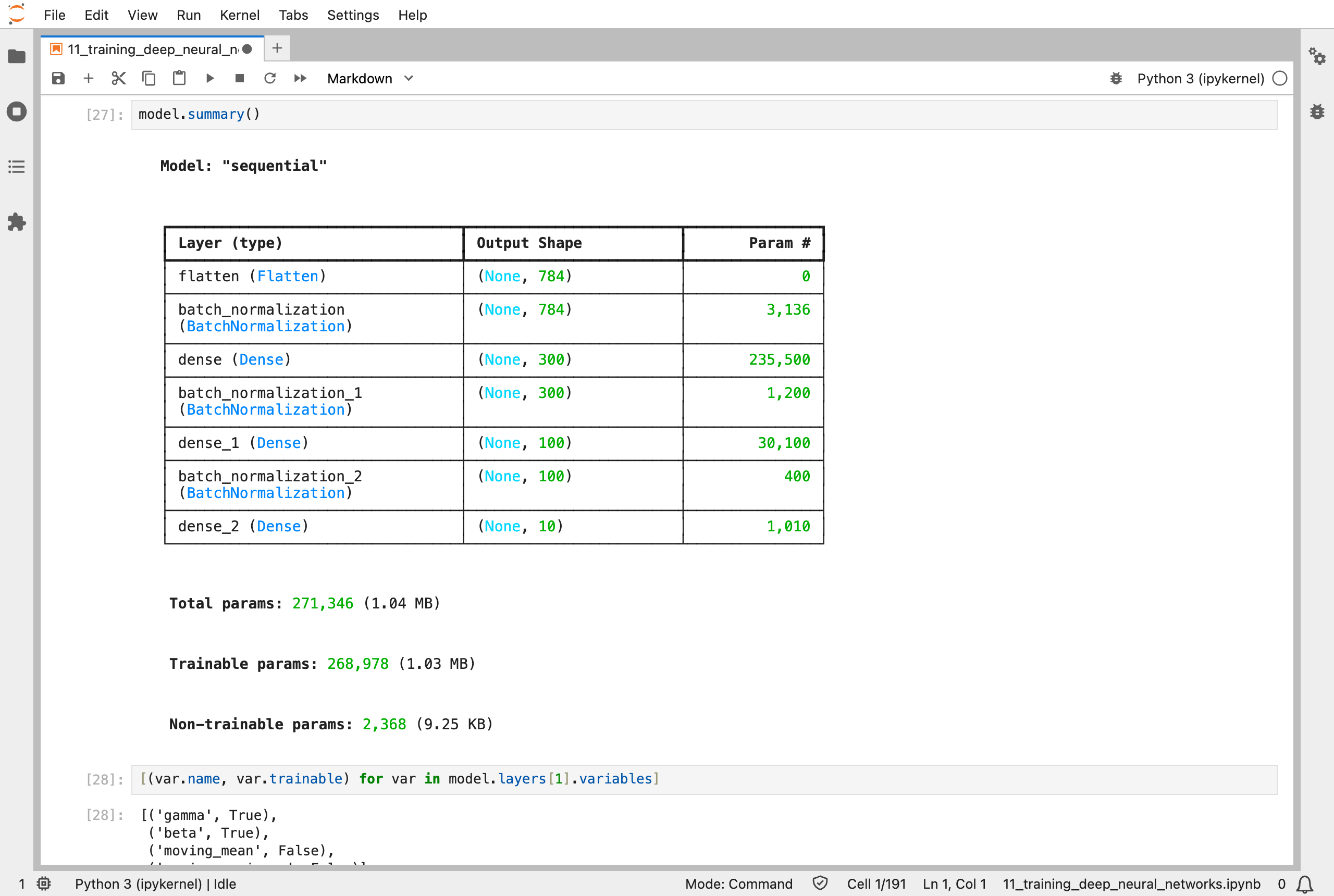
Batch normalization layers between the dense layers: 2,368 of the network's 271,346 numbers are running averages, not nudged by backpropagation

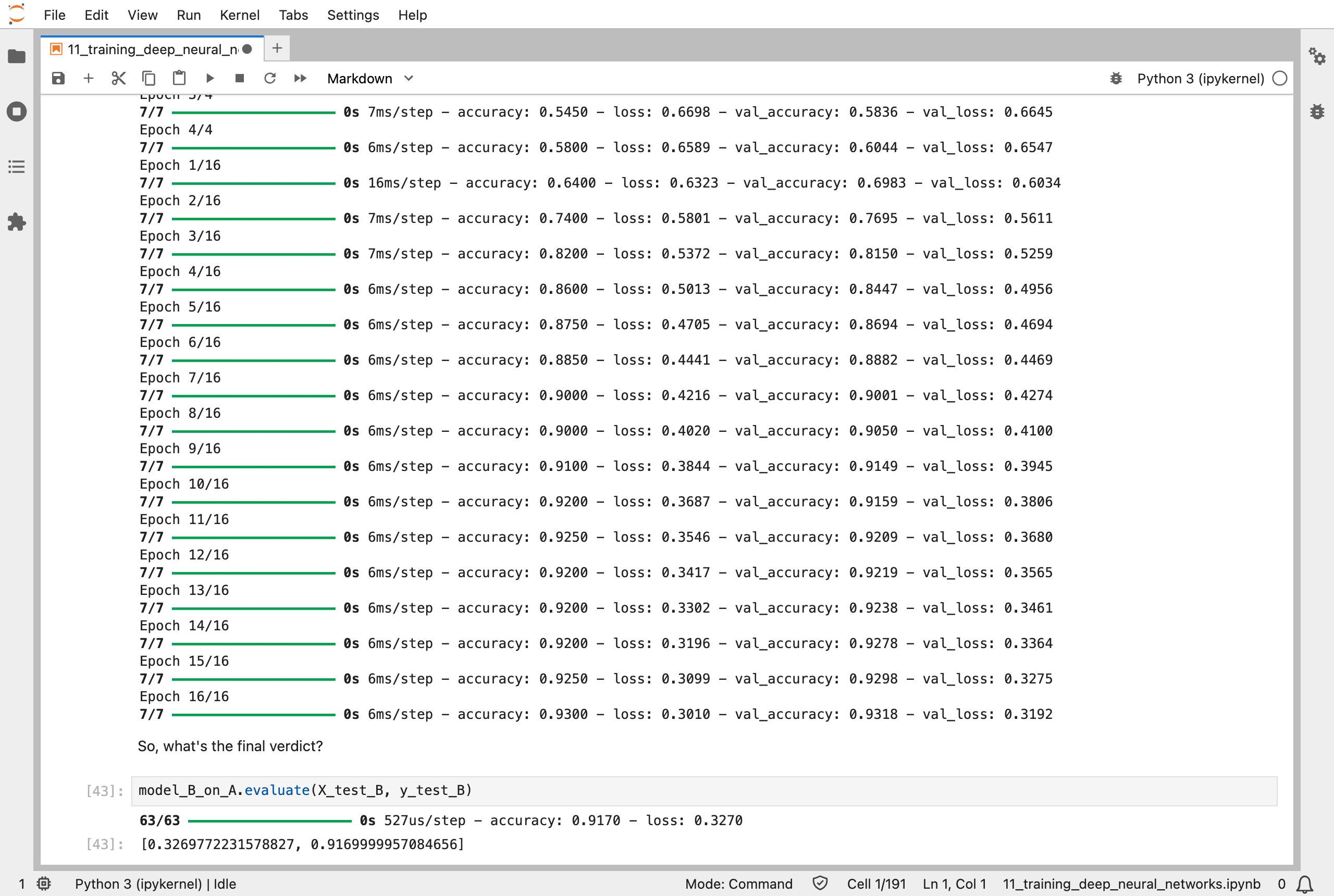
Reusing the layers of a network trained on eight other kinds of clothing: 91.7% of the test shirts and pullovers right, after training on only 200 images

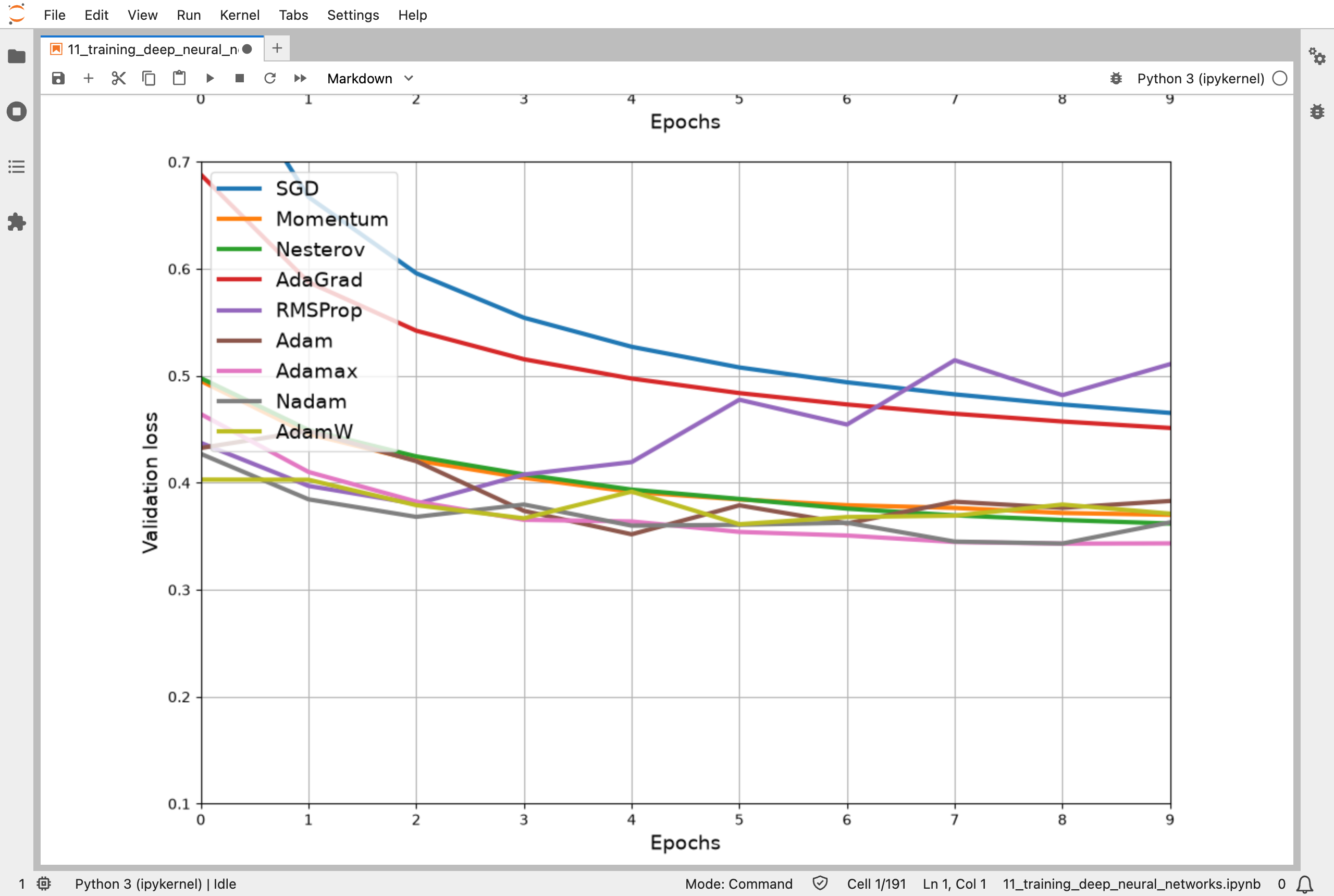
The validation loss for every optimizer: plain SGD and AdaGrad fall slowly, and RMSProp wanders back up

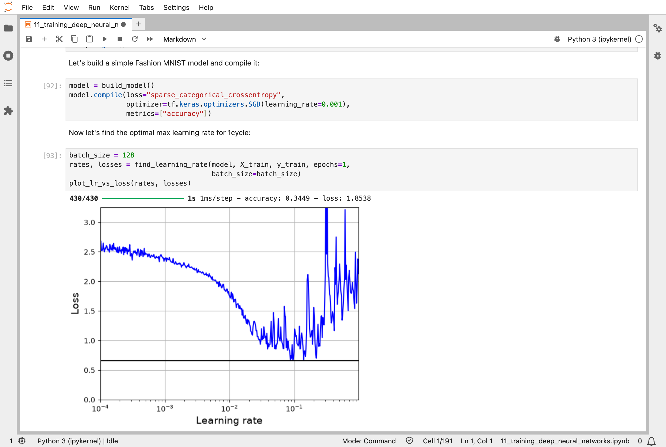
Raising the learning rate step by step during one pass: the loss falls until about 0.1, and then the training falls apart

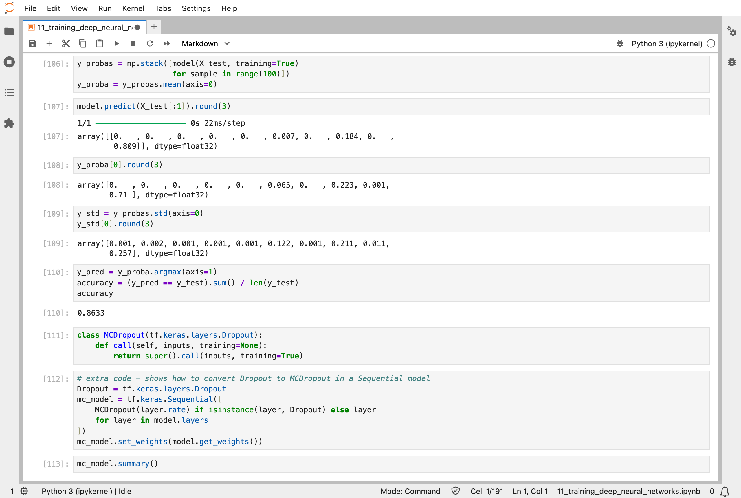
MC dropout: the average of 100 runs with dropout left on says 71% ankle boot for the first test image, where the plain network said 81%

Next, Scikit-Learn (Part 12) works through chapter 12: custom models and training with TensorFlow, where I write the training loop myself.

Scikit-Learn (Part 10)

Neural networks with Keras: a network of 266,610 numbers that learns to recognise clothing, trained by backpropagation, the way large language models are

Next in series →

Scikit-Learn (Part 12)

Custom models and training with TensorFlow: tensors, automatic slopes with GradientTape, and a training loop written by hand instead of calling fit()