Scikit-Learn (Part 4)

Neil Haddley • October 12, 2026

Training linear models: the same line worked out directly and found by gradient descent, then curves, regularization, and logistic regression

AI Pythonmachine-learningscikit-learngradient-descentlinear-regressionregularizationlogistic-regression

In Part 3, I trained a classifier without asking how it finds its numbers. This chapter of the Hands-On Machine Learning book asks. The example is made up on purpose: 100 points scattered around the line y = 4 + 3x, with random noise added, so that I know the line I am looking for. The job is to find it again from the points alone, in two completely different ways.

The first is a formula, the Normal Equation, which gives the best line in one calculation. The second is nudging: start with a random line, see which way would make it less wrong, move a little that way, and repeat. Both ended on the same line, with an intercept of 4.215 and a slope of 2.770. It is not exactly 4 and 3, because the noise pushed the points off the line.

Key Points

The lesson: nudging reaches the same answer as the formula, and nudging is the one that still works when there is no formula. For a straight line there is one. For a neural network, or my MiniGPT model, there is none, so nudging, repeated many thousands of times, is the only way. The method has a proper name, gradient descent: the slope of the error shows which way is downhill, and each step goes a little way down it.

What I learned from it:

The size of each step, called the learning rate, matters a lot: too small and the line creeps, too large and it jumps out of the valley altogether.
Nudging can use all the data for each step, one point at a time, or small groups. They all reach roughly the same line.
A "linear" model can still fit a curve, if I give it the curve as a feature: adding x² as a second column let it fit a curve close to y = 2 + x + 0.5x².

The chapter also shows how to stop a model fitting the noise, with a penalty on large numbers (regularization), and how the same idea gives chances for a classification, in logistic regression. Logistic regression appears in the notebook screenshots below, and I do not go into either here.

Quick Example

The notebook makes 100 points from the line y = 4 + 3x, plus random noise, and then looks for that line. Batch gradient descent is only a few lines of NumPy:

PYTHON

1eta = 0.1  # learning rate
2n_epochs = 1000
3m = len(X_b)  # number of instances
4
5np.random.seed(42)
6theta = np.random.randn(2, 1)  # randomly initialized model parameters
7
8for epoch in range(n_epochs):
9    gradients = 2 / m * X_b.T @ (X_b @ theta - y)
10    theta = theta - eta * gradients

Here is what each method found when I ran the notebook. Batch gradient descent uses all 100 points for every step, and stochastic gradient descent uses one point at a time. The noise means that no method can recover exactly 4 and 3:

Method	Intercept	Slope
The line used to make the data	4	3
The Normal Equation, in one calculation	4.215	2.770
Batch gradient descent, 1,000 steps from random numbers	4.215	2.770
Stochastic gradient descent, 50 passes through the data	4.211	2.749
Scikit-Learn's `SGDRegressor`	4.213	2.773

What training means here

Nudging first appeared in Part 3, where the SGDClassifier learned by it, and this is the chapter that explains it. The loop above is the whole idea: start from two random numbers, work out which way the error slopes, take a small step downhill, and repeat. After 1,000 steps it lands on exactly the line that the Normal Equation works out in one go.

Two differences from my MiniGPT model are worth seeing. The slope here comes from a formula worked out by hand once, 2 / m * X_b.T @ (X_b @ theta - y), because a linear model has only one layer; MiniGPT has many layers, so PyTorch has to work its slopes out by backpropagation. And here there are 2 numbers to nudge, where MiniGPT has 826,433. The step itself is the same: a number minus the learning rate times its slope.

The SGDClassifier in Part 3 trains in exactly this way, and so does a neural network. The rest of the models in this series so far are either worked out directly, like the Normal Equation, or grown one decision at a time, like decision trees.

There are no Dumb Questions

Q: Why use gradient descent, when the Normal Equation gives the answer directly?

A: For a line through points with one measurement, such as age, the Normal Equation is the school-level calculation and is instant. A "feature" is one measurement for each point, one column of the data table, and with many features the same formula needs a bigger table: it works with a square table with one row and one column for every feature, and has to invert it. Two features make a 2 × 2 table, which is trivial. A thousand features make a table with a million entries, and the work to invert a table grows roughly with the cube of its side, so doubling the features makes the work about eight times bigger. On my Mac, with 20,000 rows of random data, the whole calculation took 0.012 seconds for 100 features, 0.37 seconds for 1,000, and 3.3 seconds for 4,000. At 100,000 features the table alone would hold ten billion numbers, about 80 gigabytes, which will not fit in memory. Gradient descent never builds that table. Each step does an amount of work in proportion to the number of features, so it carries on working when the formula cannot. And for most models, such as neural networks, there is no formula at all, so nudging is the only way.

Pictures and text have thousands to millions of features: a single 1,000 × 1,000 pixel photo has a million. That is where the formula stops being practical.

Q: What is an epoch?

A: One pass through the training data. Batch gradient descent uses all 100 points for every step, so its 1,000 epochs are 1,000 steps. Stochastic gradient descent takes one step per point, so its 50 epochs are 5,000 smaller, noisier steps.

Q: Why did the different methods not all find exactly 4 and 3?

A: The points have random noise added, so the best line through these 100 points is not quite y = 4 + 3x. The Normal Equation and batch gradient descent both found that best line, 4.215 and 2.770; the stochastic methods finished close to it.

Running the notebook in Jupyter

The chapter is in the notebook that goes with the book, 04_training_linear_models.ipynb. I ran everything before the exercise solutions, which took a few seconds on my Mac Studio, and then looked through the results in JupyterLab.

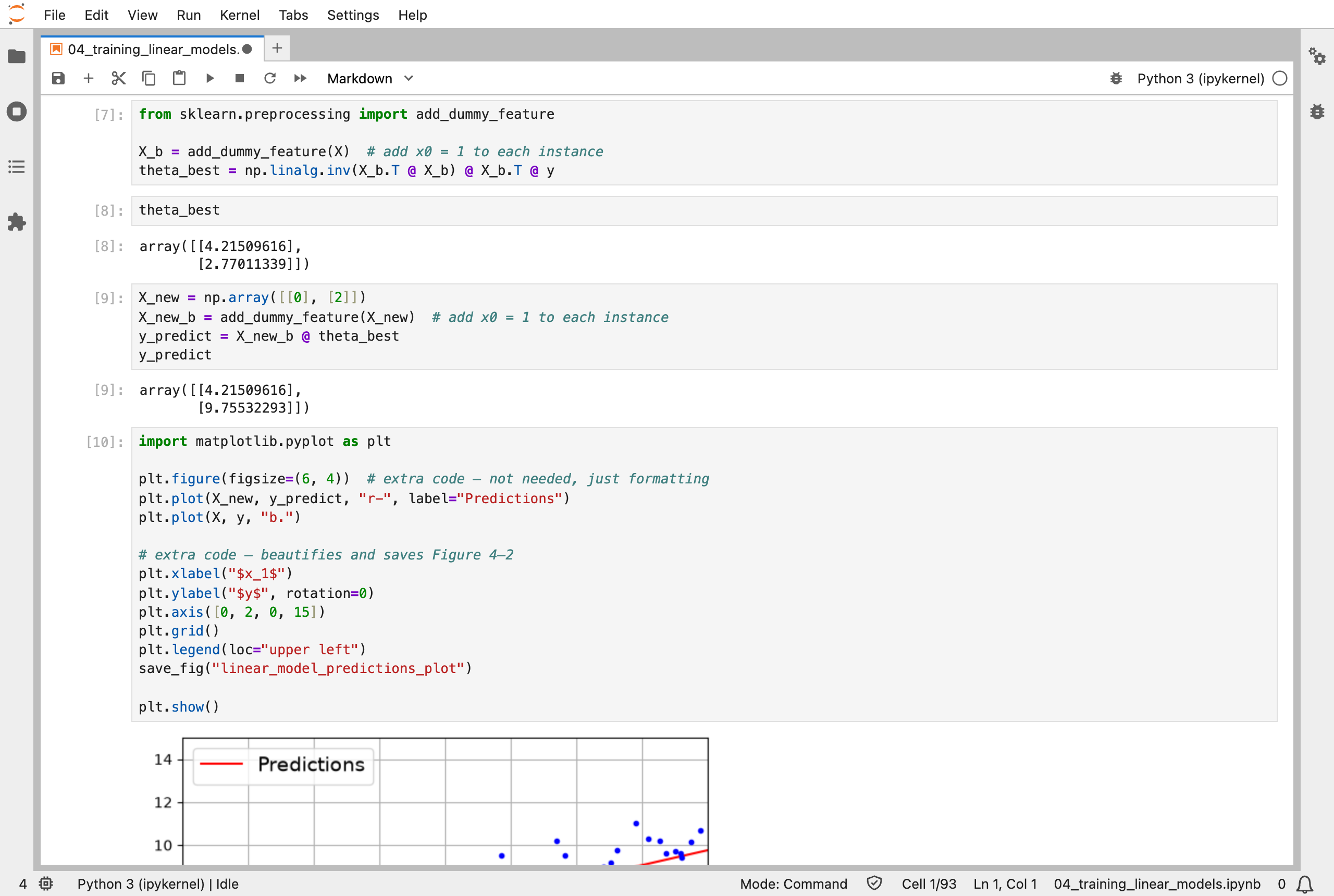
I worked out the best line directly, with the Normal Equation: an intercept of 4.215 and a slope of 2.770, close to the 4 and 3 used to make the data

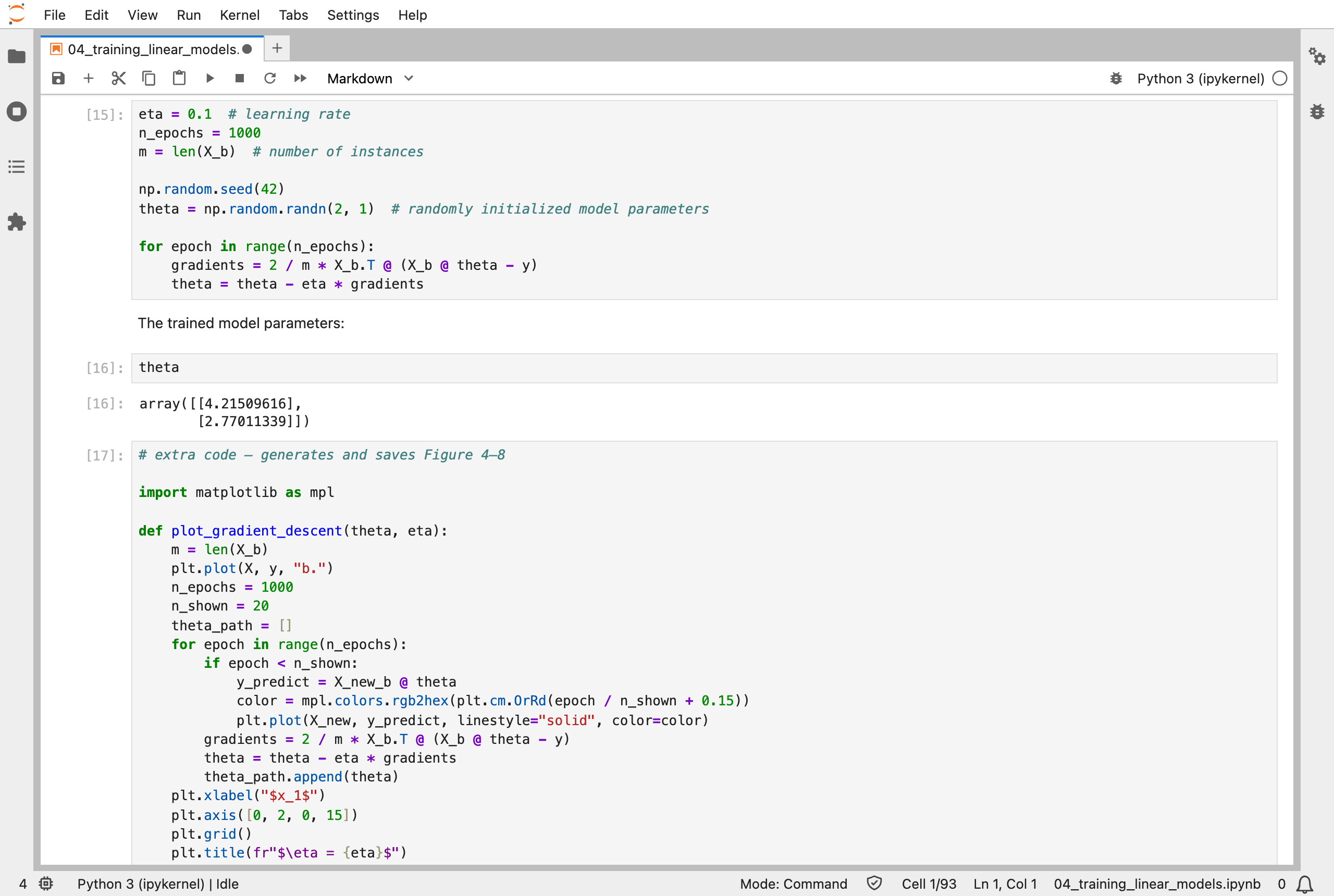
Batch gradient descent started from random numbers, took 1,000 steps downhill, and arrived at exactly the same 4.215 and 2.770

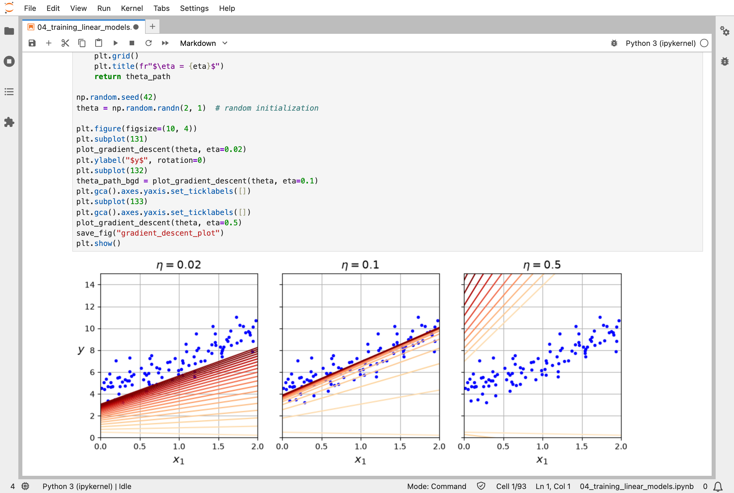
The first 20 steps with three learning rates: 0.02 creeps towards the line, 0.1 gets there, and 0.5 overshoots and flies away

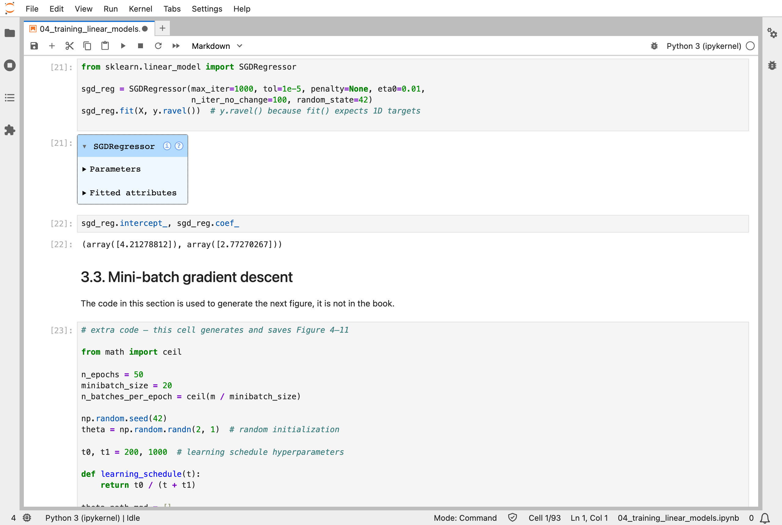
Scikit-Learn's SGDRegressor does the same nudging, one instance at a time, and found 4.213 and 2.773

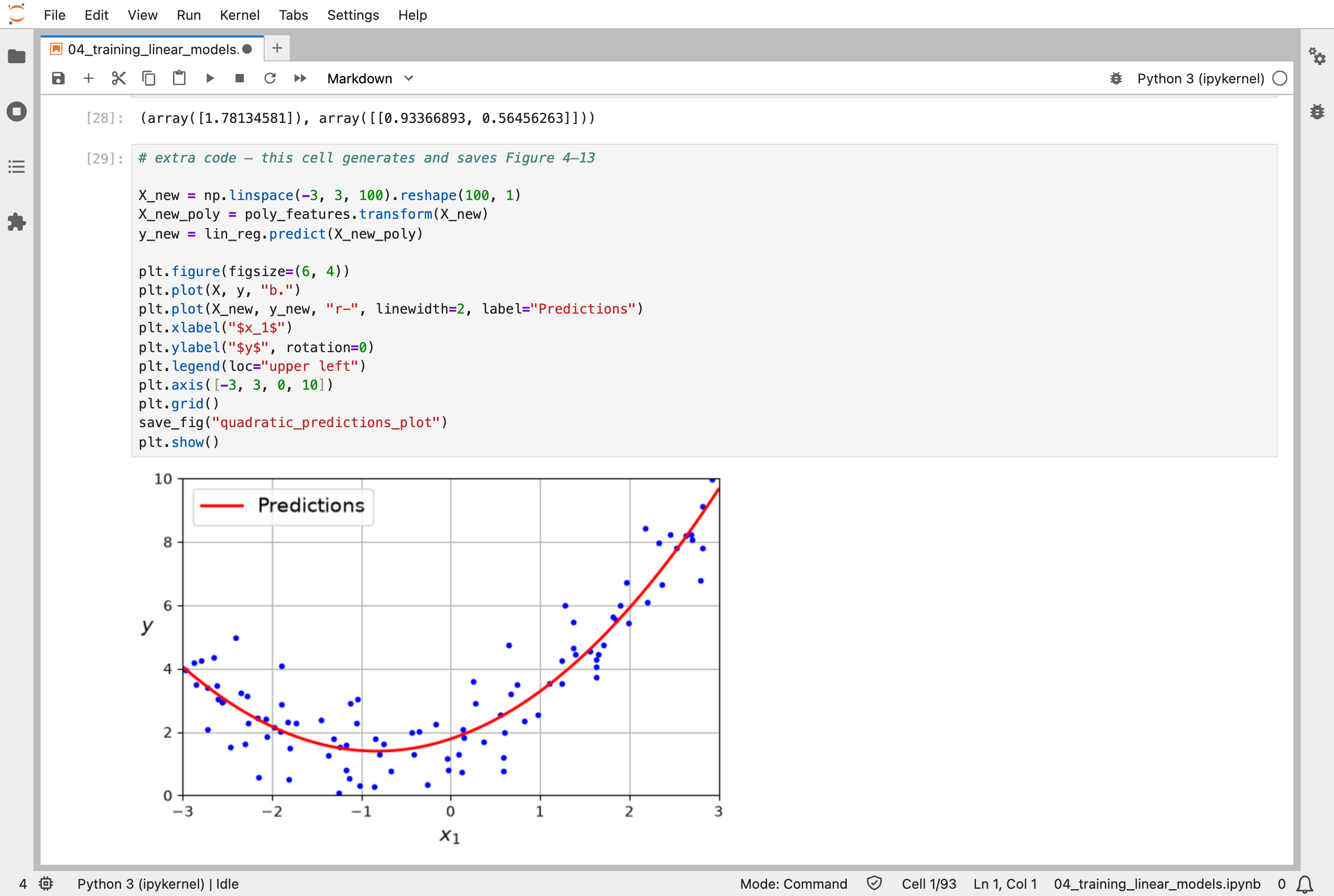
Adding x² as a second feature lets a linear model fit a curve: 1.78 + 0.93x + 0.56x², close to the 2 + x + 0.5x² used to make the data

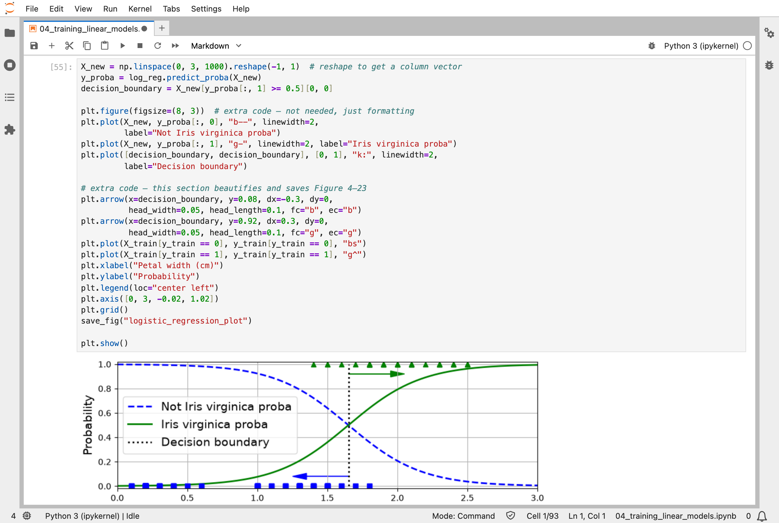
Logistic regression on iris petals: above a petal width of about 1.65 cm, it says Iris virginica is more likely than not

Next, Scikit-Learn (Part 5) works through chapter 5: support vector machines.

Scikit-Learn (Part 3)

Classification: recognising handwritten digits, and why accuracy alone can mislead, with confusion matrices, precision, and recall

Next in series →

Scikit-Learn (Part 5)

Support vector machines: the widest street between two classes, kernels for curved boundaries, and an SVM trained both directly and by gradient descent