In Part 9, I found groups in data with no labels. This chapter of the Hands-On Machine Learning book starts the second half of the book, on neural networks, the models behind most of today's AI, including the large language models behind tools like ChatGPT. I build them with Keras, a library that sits on top of TensorFlow, and train them with backpropagation.
The task is real, if small: look at a 28 × 28 picture of an item of clothing, one of 70,000 in a set called Fashion MNIST, and say which of 10 kinds it is, from T-shirts to ankle boots. My network was right on 87.4% of 10,000 test pictures it had never seen. It had 266,610 numbers, and it learned all of them from the training pictures.
Key Points
The lesson: a neural network is not a new kind of mathematics. It is layers of the weighted sums from earlier parts, with a simple bend between each layer, so that the network can learn curved patterns and not only straight ones. Its numbers start at random, and are nudged, a little at a time, in the direction that makes the answers less wrong. Backpropagation is how it works out that direction for every number in every layer at once.
What I learned from it:
- The bend between layers is a simple rule, such as "replace negative numbers with zero" (called ReLU, for rectified linear unit). Without it, a hundred layers would be no better than one.
- The settings that shape a network, such as how many layers, how many neurons in each, and how big each nudge is, are mostly found by trying them, not worked out. The notebook automates the trying.
- A network can be built as an ordered stack of layers, which is what I did, or in more flexible ways for networks with several inputs or outputs.
The chapter also covers the history of artificial neurons, saving a trained network, and stopping training early when it stops improving. I do not go into those here.
Quick Example
A classifier for Fashion MNIST, 70,000 small images of clothing in 10 classes, from T-shirts to ankle boots. Each 28 × 28 image is flattened to 784 numbers, and passes through layers of 300, 100, and 10 neurons:
PYTHON
1import tensorflow as tf
2
3model = tf.keras.Sequential([
4    tf.keras.layers.Flatten(input_shape=[28, 28]),
5    tf.keras.layers.Dense(300, activation="relu"),
6    tf.keras.layers.Dense(100, activation="relu"),
7    tf.keras.layers.Dense(10, activation="softmax")
8])
9model.compile(loss="sparse_categorical_crossentropy",
10              optimizer="sgd",
11              metrics=["accuracy"])
12history = model.fit(X_train, y_train, epochs=30,
13                    validation_data=(X_valid, y_valid))
Here is what the networks did when I ran the notebook:
| Network | Result |
|---|---|
| Clothing classifier, 266,610 numbers, after 30 passes through 55,000 images | 87.4% of the 10,000 test images right |
| Its first three test images | ankle boot, pullover, trouser: all three right |
California house prices, Scikit-Learn's MLPRegressor | a typical error (RMSE, as in Part 2) of 0.505, about $50,500 |
| California house prices, a Keras network | a typical error (RMSE) of 0.535, about $53,500 |
| Automatic search for the best network size and step size, 60 trials | best validation accuracy 86.6% |
What training means here
This is backpropagation, and it is the same recipe that trains my MiniGPT model.
The clothing classifier's 266,610 numbers start at random (its biases start at zero). Each training step takes 32 images, runs them through the network, and scores how surprised the network was by the right answers: that is the sparse_categorical_crossentropy loss, the surprise score from MiniGPT. Then TensorFlow works backwards through every layer to find the slope for each of the 266,610 numbers, and plain gradient descent, "sgd", nudges each one a little, with a learning rate of 0.01. One pass through the 55,000 training images is 1,719 such steps, and the network makes 30 passes: 51,570 nudges in all.
MiniGPT is the same machine at a different scale: 826,433 numbers, 3,000 steps of 32 snippets of text, AdamW instead of plain gradient descent, and attention layers between the dense ones. Scikit-Learn's MLPRegressor, the first network in this chapter, is trained by backpropagation too.
Here is how training has changed through this series:
| Parts | How the models learn |
|---|---|
| 1, 2 | worked out exactly (the best straight line), remembered (k-nearest neighbors), or grown one split at a time (trees and forests) |
| 3, 4 | nudged by gradient descent, with slopes from a formula, because the models have one layer |
| 5 | solved directly by a specialised solver, or by gradient descent, which reaches almost the same answer |
| 6, 7 | trees grown greedily, and combined into ensembles; gradient boosting steps downhill by adding trees |
| 8, 9 | no labels: PCA (principal component analysis) is worked out, K-Means alternates between two exact steps, and t-SNE (t-distributed stochastic neighbor embedding) nudges points |
| 10 | many layers, so the slopes come from backpropagation, and every number is nudged |
Running the notebook in Jupyter
The chapter is in the notebook that goes with the book, 10_neural_nets_with_keras.ipynb. I ran everything before the exercise solutions, which took about 14 minutes on my Mac Studio, most of it in the three hyperparameter searches, and then looked through the results in JupyterLab. I could not open TensorBoard, the separate viewer for the training logs, so I have left that part out.
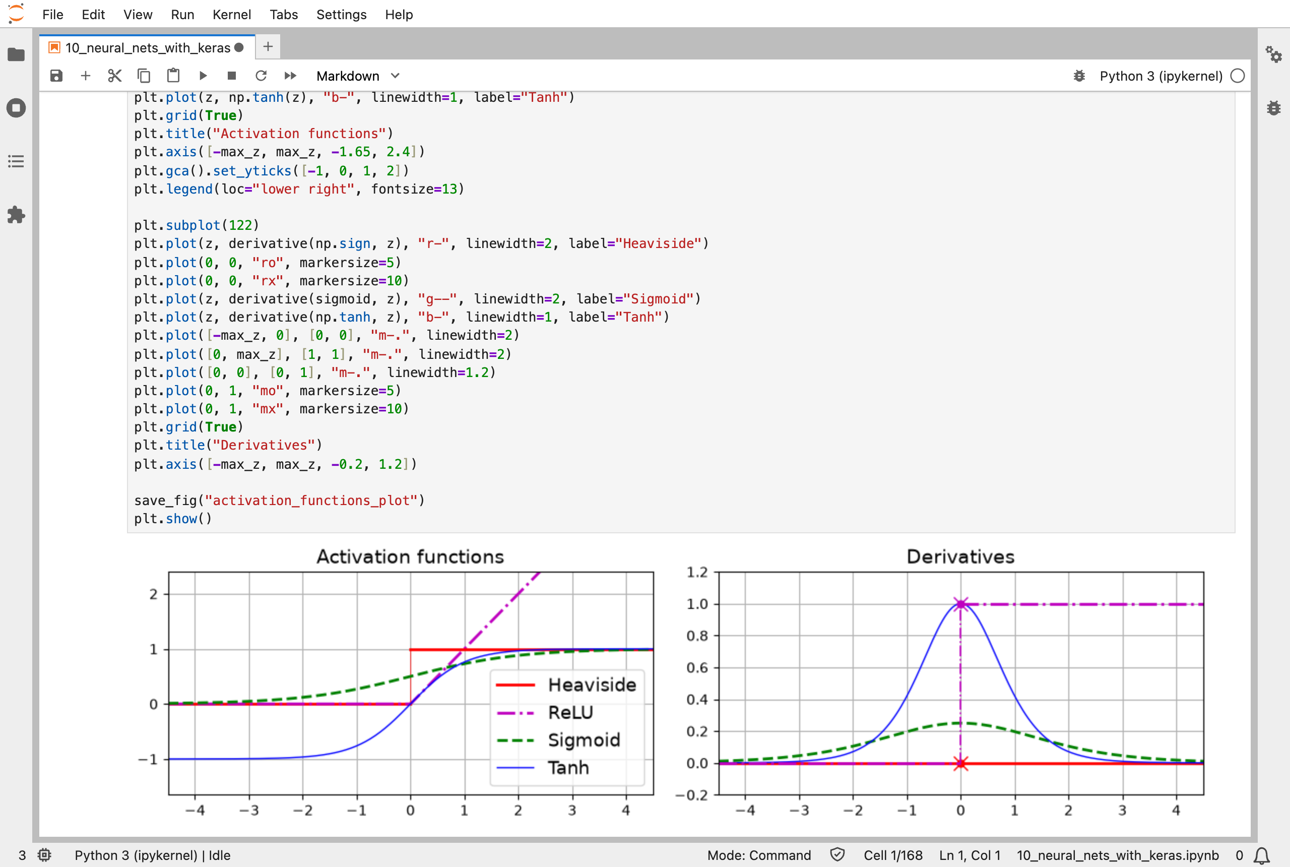
Activation functions, the bends between layers: the step function of the original perceptron, ReLU, sigmoid, and tanh, with their slopes on the right
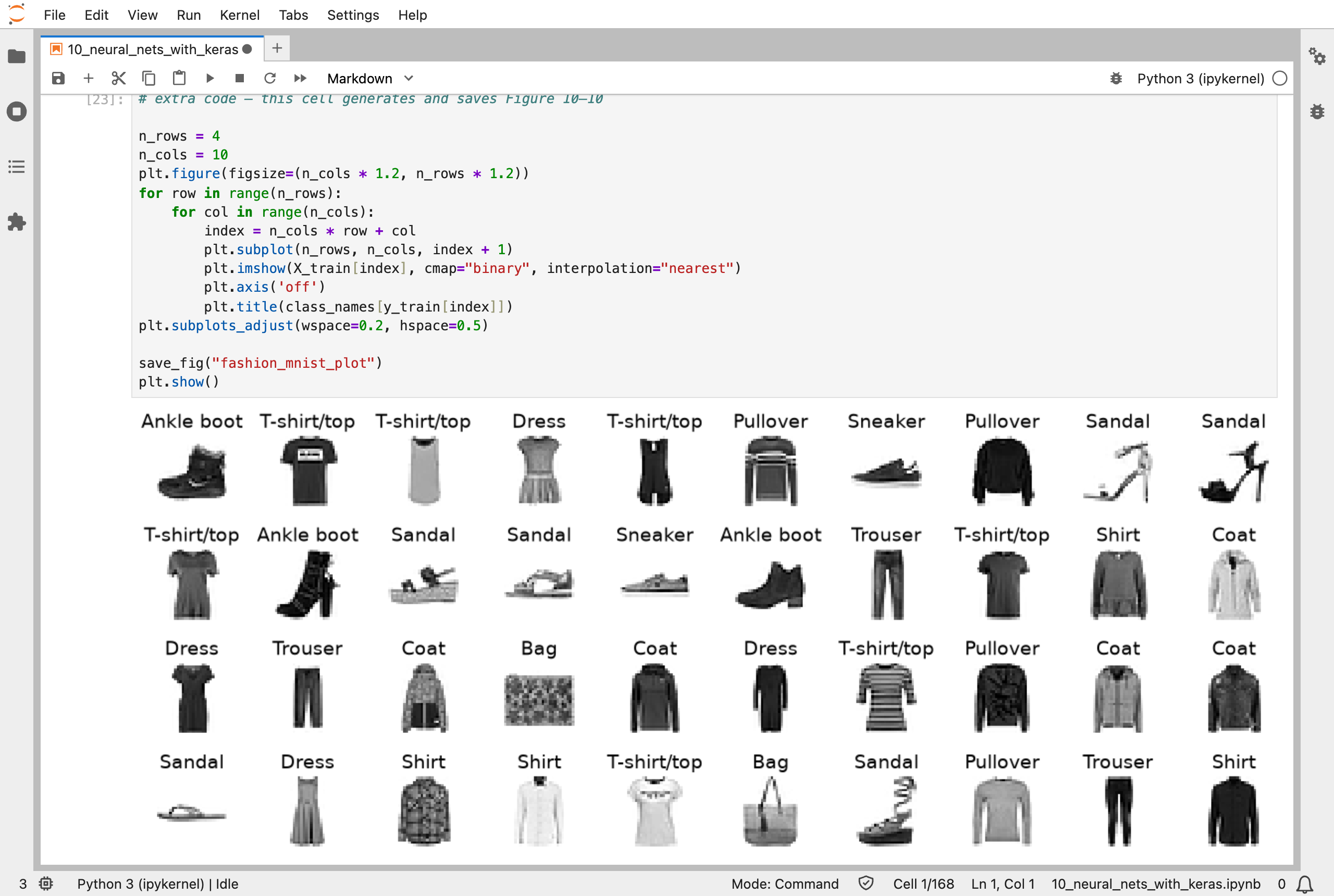
A sample of Fashion MNIST: 28 × 28 images of clothing, each labelled with one of 10 classes
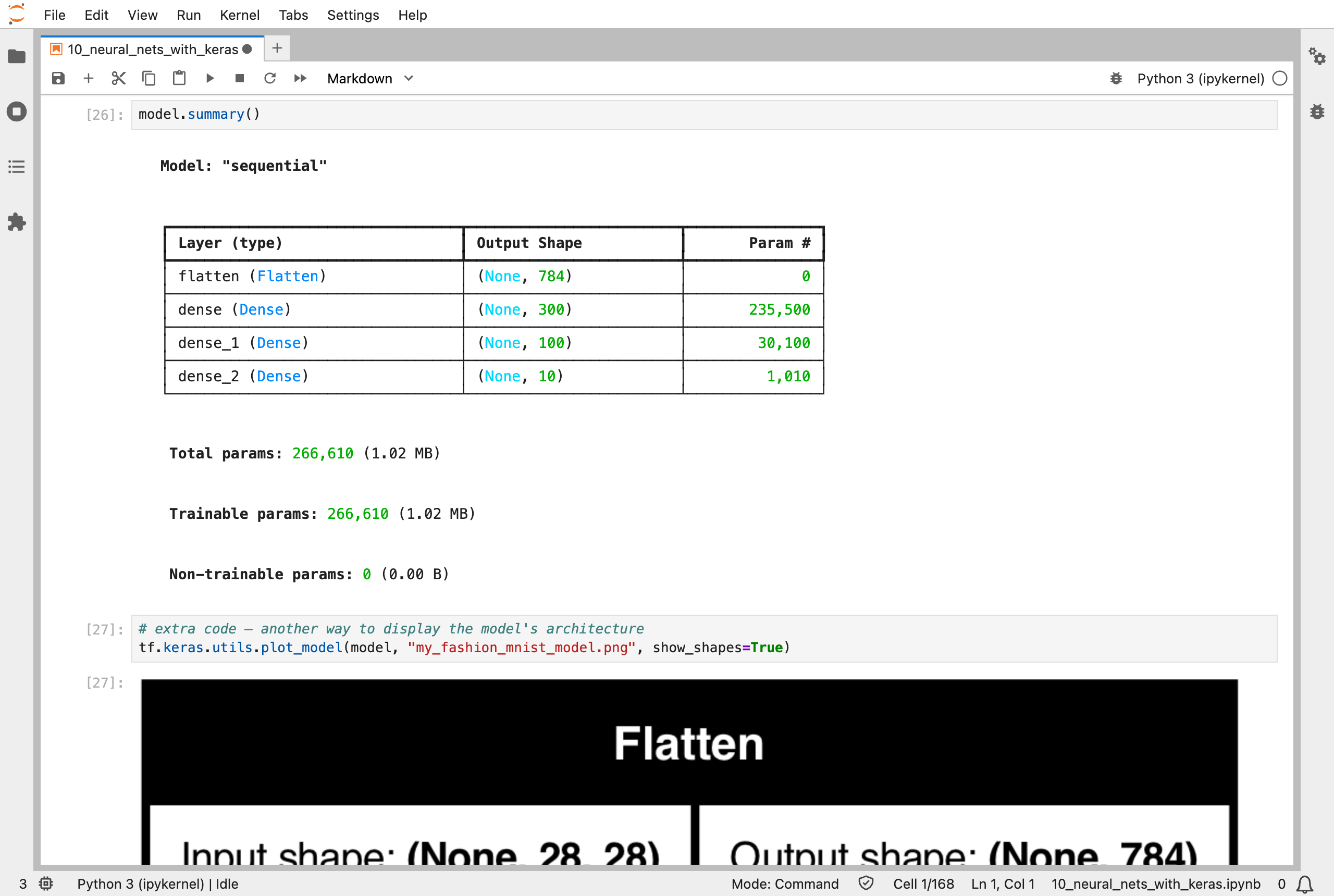
The network's layers: 235,500 numbers in the first hidden layer, 30,100 in the second, and 1,010 in the output layer, 266,610 in all
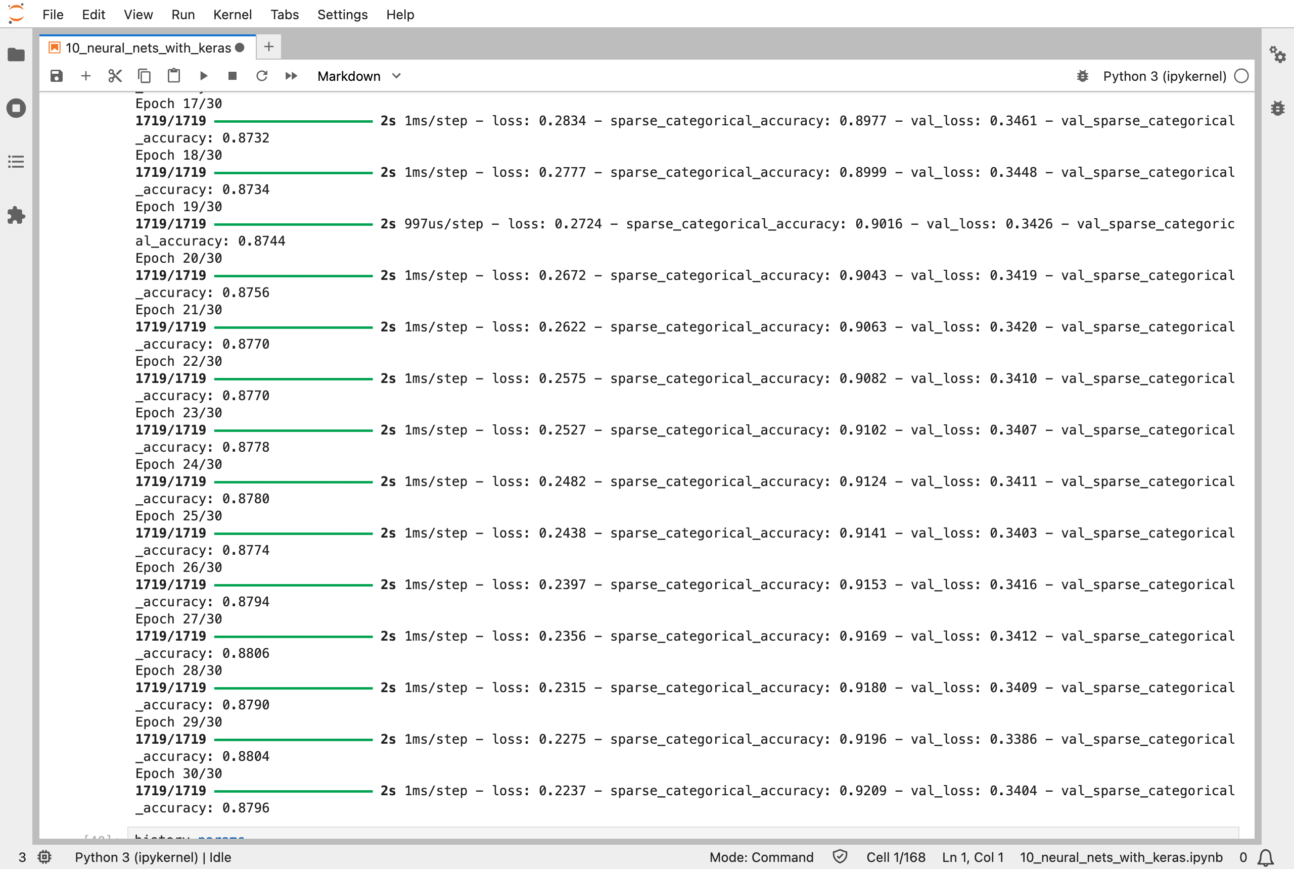
The end of training: after 30 passes, about 92% of the training images and 88% of the validation images are right
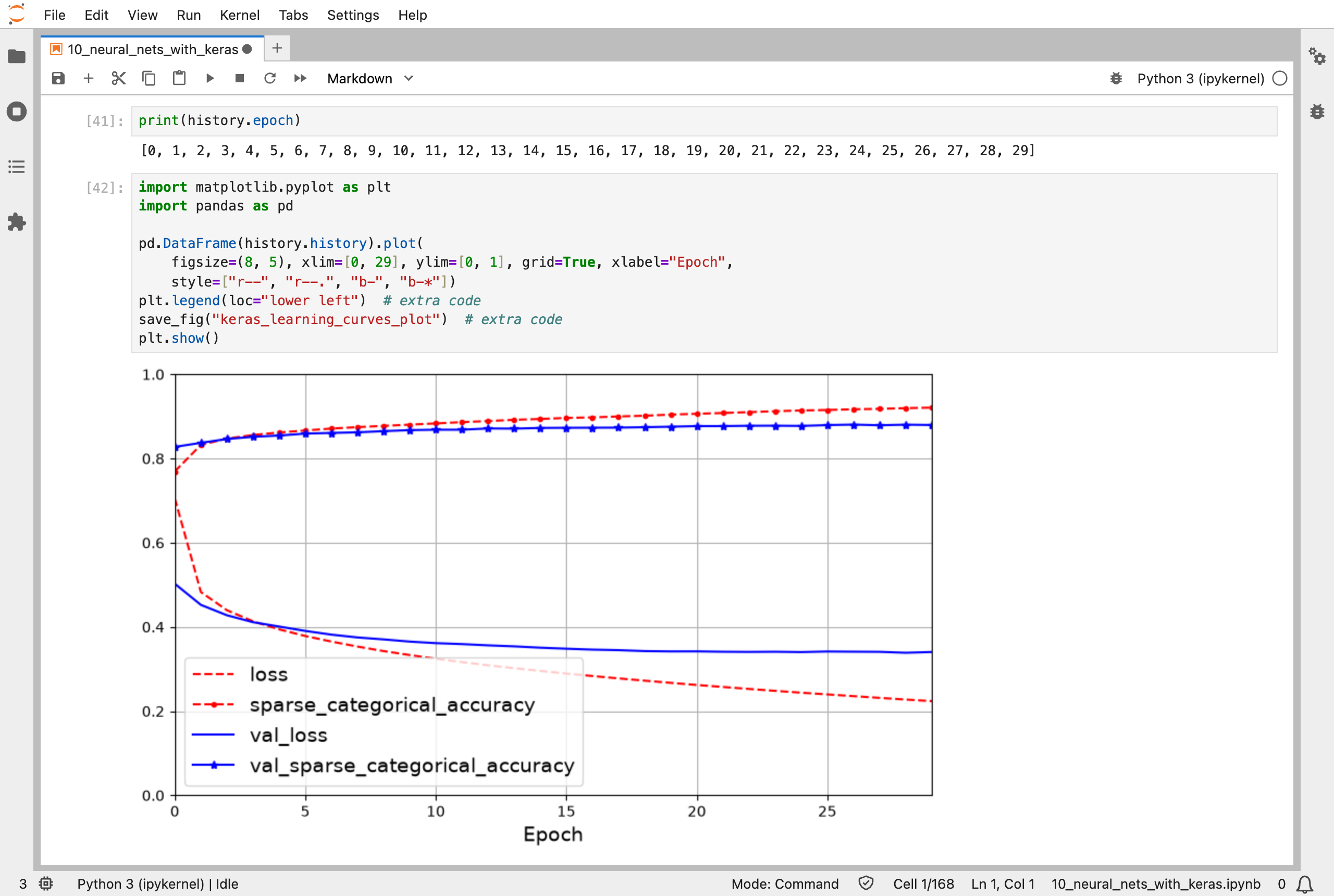
The learning curves: the loss falls and the accuracy rises, epoch by epoch, and the training and validation curves slowly move apart
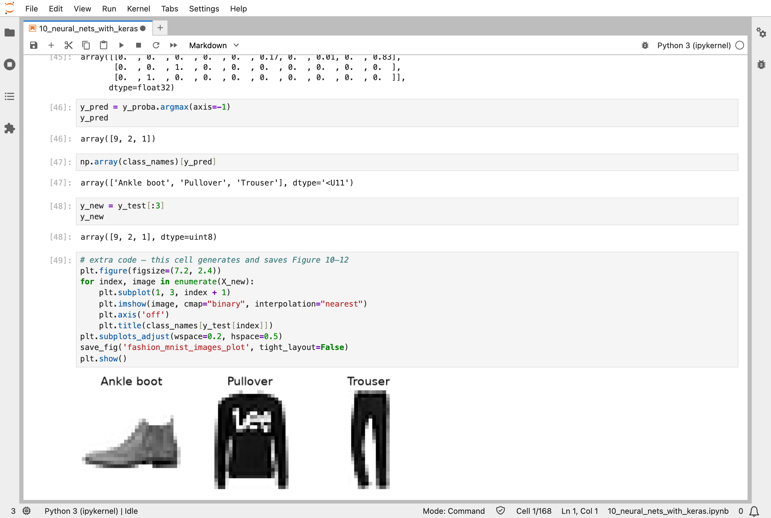
The network's predictions for the first three test images: an ankle boot, a pullover, and a trouser, all correct
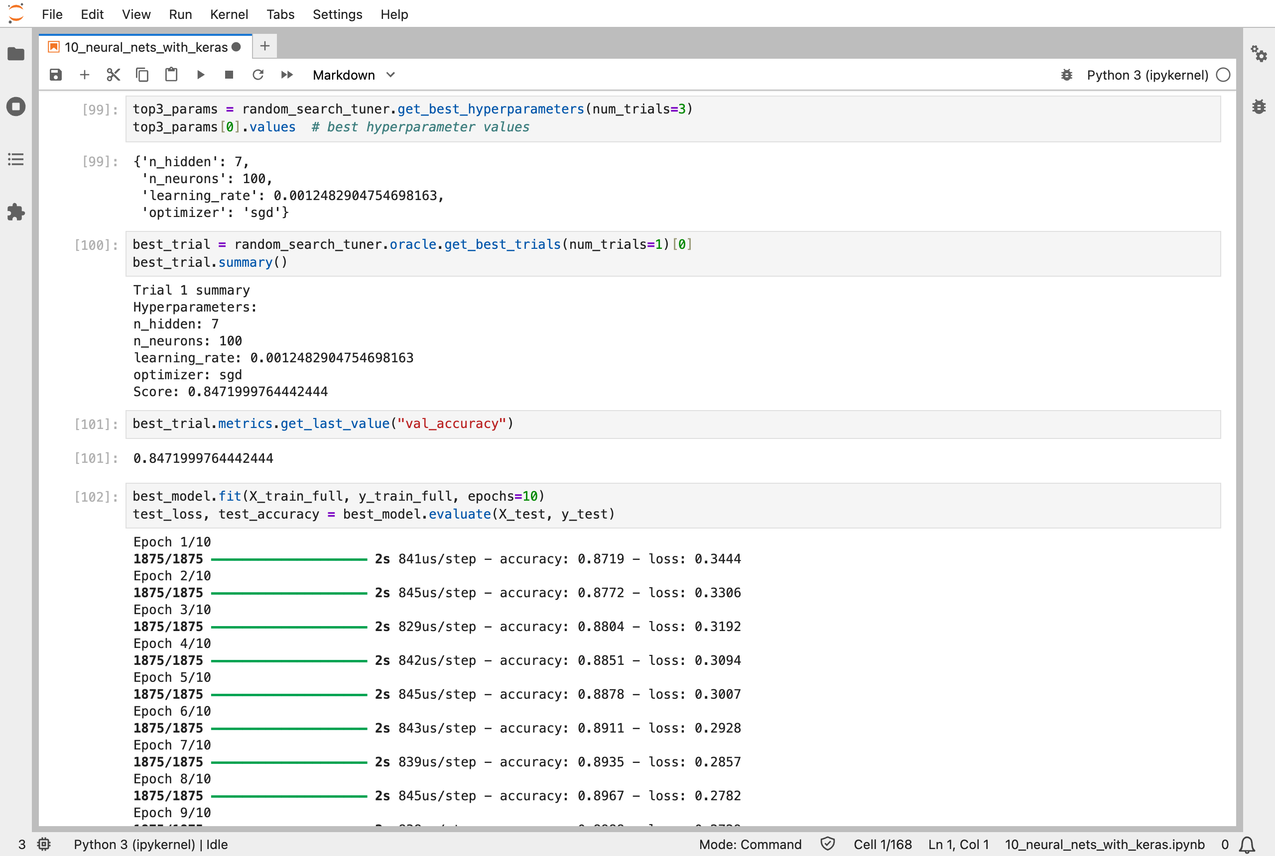
Keras Tuner's random search: its best network had 7 hidden layers of 100 neurons, and 84.7% validation accuracy
Next, Scikit-Learn (Part 11) works through chapter 11: training deep neural networks, and the tricks that make deep networks trainable.