Scikit-Learn (Part 15)
Neil Haddley • October 13, 2026
Processing sequences with recurrent neural networks (RNNs) and CNNs: forecasting daily train ridership, comparing a naive guess, a statistical model, and RNNs, and forecasting several days ahead
In Part 14, a convolutional network looked at a picture. This chapter of the Hands-On Machine Learning book is about data in which the order matters: a sequence, such as one number for each day. The task is real. The Chicago Transit Authority publishes how many people board its trains and buses every day, and the job is to forecast tomorrow's train boardings from the last 56 days. A model's score is its average error, in boardings per day.
Before building anything clever, the notebook tries the simplest forecast: "the same as one week earlier". It was off by 42,143 boardings per day on average, out of roughly 700,000 on a weekday. The best network was off by 24,021, which is about 40% better. A network with a single neuron was off by 102,752, worse than doing nothing clever. Without the simple forecast to compare against, I would not have known it was bad.
Key Points
The lesson: work out what a simple guess scores before building a model, because it is hard to beat by much, and it tells me whether a clever model is worth having. The networks in this chapter, called recurrent networks, read a window of days one at a time, carrying a memory forward from each day to the next, with the same numbers at every step. In my run the best result came from giving the network more to look at: the bus counts and the type of the next day, as well as the train counts.
What I learned from it:
- A statistical forecasting method called SARIMA, which models weekly patterns directly, scored 32,041, close to the network's 29,979 on the train counts alone. For a small problem like this, a simpler model is often nearly as good.
- Forecasting several days ahead by feeding the model its own forecasts makes errors pile up. Training it to forecast all 14 days at once avoids that: its error grew from 23,219 for tomorrow to between 32,000 and 38,000 from the fifth day onwards.
- The more elaborate memory cells in the chapter, LSTM (long short-term memory) and GRU (gated recurrent unit), only ran for five passes, so my numbers for them are not a fair comparison.
The chapter also covers one-dimensional convolutions and a design called WaveNet for sequences, which I do not go into.
Quick Example
The data is the Chicago Transit Authority's daily boarding totals, for buses and for trains, from 2001. The notebook trains on 2016 to 2018, and checks its models on January to May 2019. Every model gets a window of the last 56 days and forecasts the next day's train boardings. This is the first RNN model that worked well:
PYTHON
1univar_model = tf.keras.Sequential([
2    tf.keras.layers.SimpleRNN(32, input_shape=[None, 1]),
3    tf.keras.layers.Dense(1)
4])
One SimpleRNN layer of 32 neurons reads the 56 days one at a time, and one ordinary neuron turns what it remembers into a forecast. The score is the mean absolute error (MAE): the average number of boardings by which the forecast is wrong, per day. Here is how each approach did when I ran the notebook:
| Forecast | Average error per day (boardings) |
|---|---|
| Naive: the same as one week earlier | 42,143 |
| SARIMA, retrained every day (statistical) | 32,041 |
| Linear model on the last 56 days | 37,674 |
One SimpleRNN neuron | 102,752 |
SimpleRNN with 32 neurons | 29,979 |
Three stacked SimpleRNN layers of 32 | 30,425 |
SimpleRNN with 5 inputs: bus, rail, and tomorrow's day type | 24,021 |
The naive and SARIMA figures are for March to May 2019, and the others for January to May 2019, so they are not exactly comparable, but they show the picture. Boardings are around 700,000 on a weekday, so an error of 24,000 is about 3% to 4%, and the naive forecast's 42,000 is about 6%. The 5-input model is the best: besides the rail history, it sees the bus history and the type of the next day, which tells it whether to expect a weekday or a weekend.
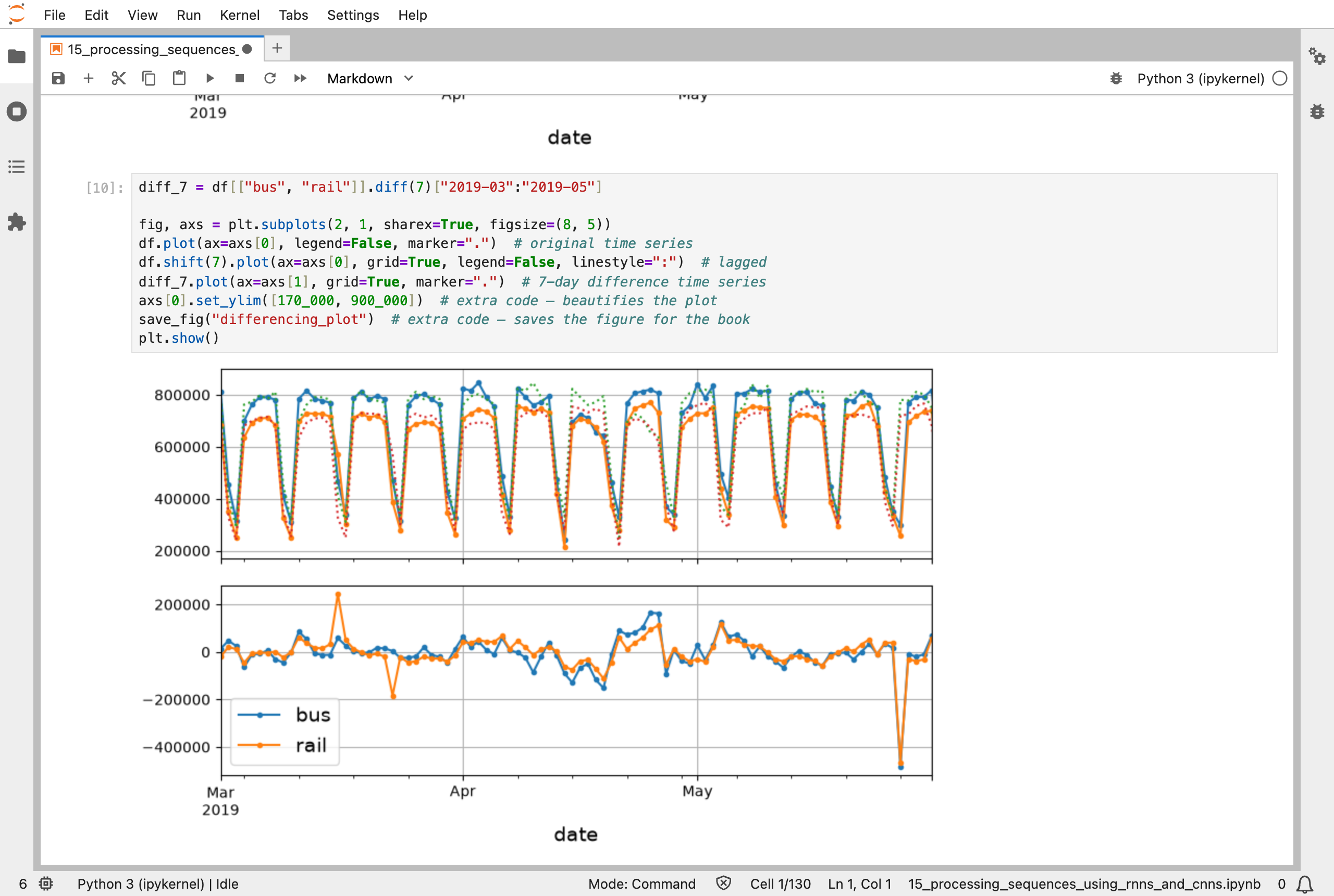
The naive forecast: the dotted line is the series moved forward by 7 days, and below it, the difference between the two lines is mostly small, apart from holidays such as Memorial Day at the end of May
What training means here
The RNN learns with the same loop as everything else in this series: a batch of windows goes in, the loss is measured, slopes are found by backpropagation, and every number is nudged. The new part is what the backward step has to cross. An RNN reads 56 days one at a time, using the same numbers at every step, so the slopes have to travel back through all 56 steps. The book calls this backpropagation through time. A long run of steps is also why RNNs are hard to train: the slopes can shrink to almost nothing or grow wildly, the problem from Part 11, and why the chapter introduces LSTM and GRU cells and layer normalization.
The data pipeline from Part 13 does the cutting. timeseries_dataset_from_array turns a series into overlapping windows, and the notebook shows how the same idea works step by step with a series of the numbers 0 to 5. Each window becomes one training example, with the next day as its target.
My MiniGPT model is also trained to predict what comes next in a sequence, but it reads its letters with attention instead of a memory carried forward, and every position is looked at in the same step. Part 16 is about both ways of reading text.
Running the notebook in Jupyter
The chapter is in the notebook that goes with the book, 15_processing_sequences_using_rnns_and_cnns.ipynb. I ran everything before the exercise solutions, which took under 10 minutes on my Mac Studio, and then looked through the results in JupyterLab. The notebook trains most models for up to 500 epochs with early stopping, which stops when the validation error has not improved for 50 epochs. But for the LSTM, GRU, layer-normalization, convolutional, and WaveNet models it trains only 5 epochs, "to show that it works", as the notebook says, so their errors, between 96,000 and 145,000, are not a fair comparison with the others.
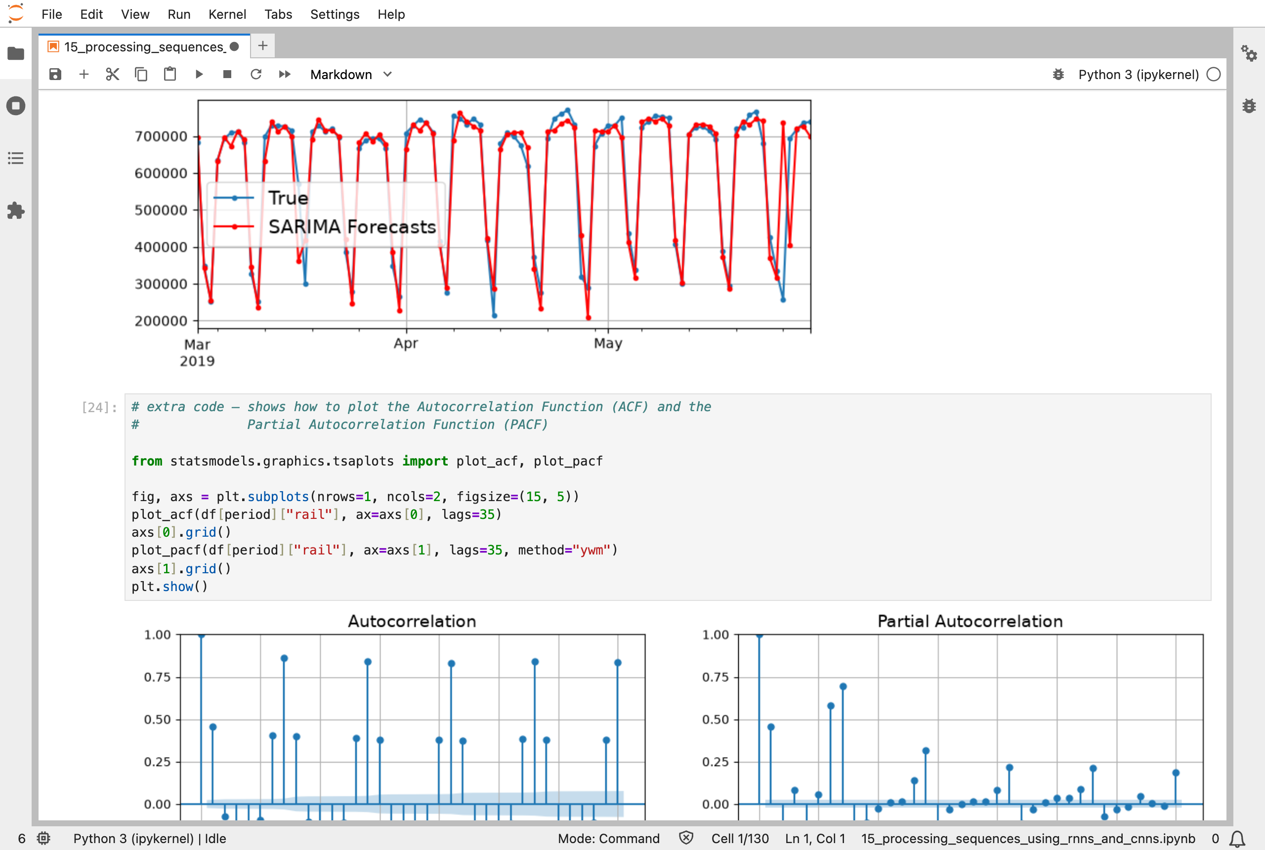
SARIMA forecasts for the validation period, retrained every day: the red forecasts follow the blue true values closely, and the autocorrelation plots below show the strong weekly pattern
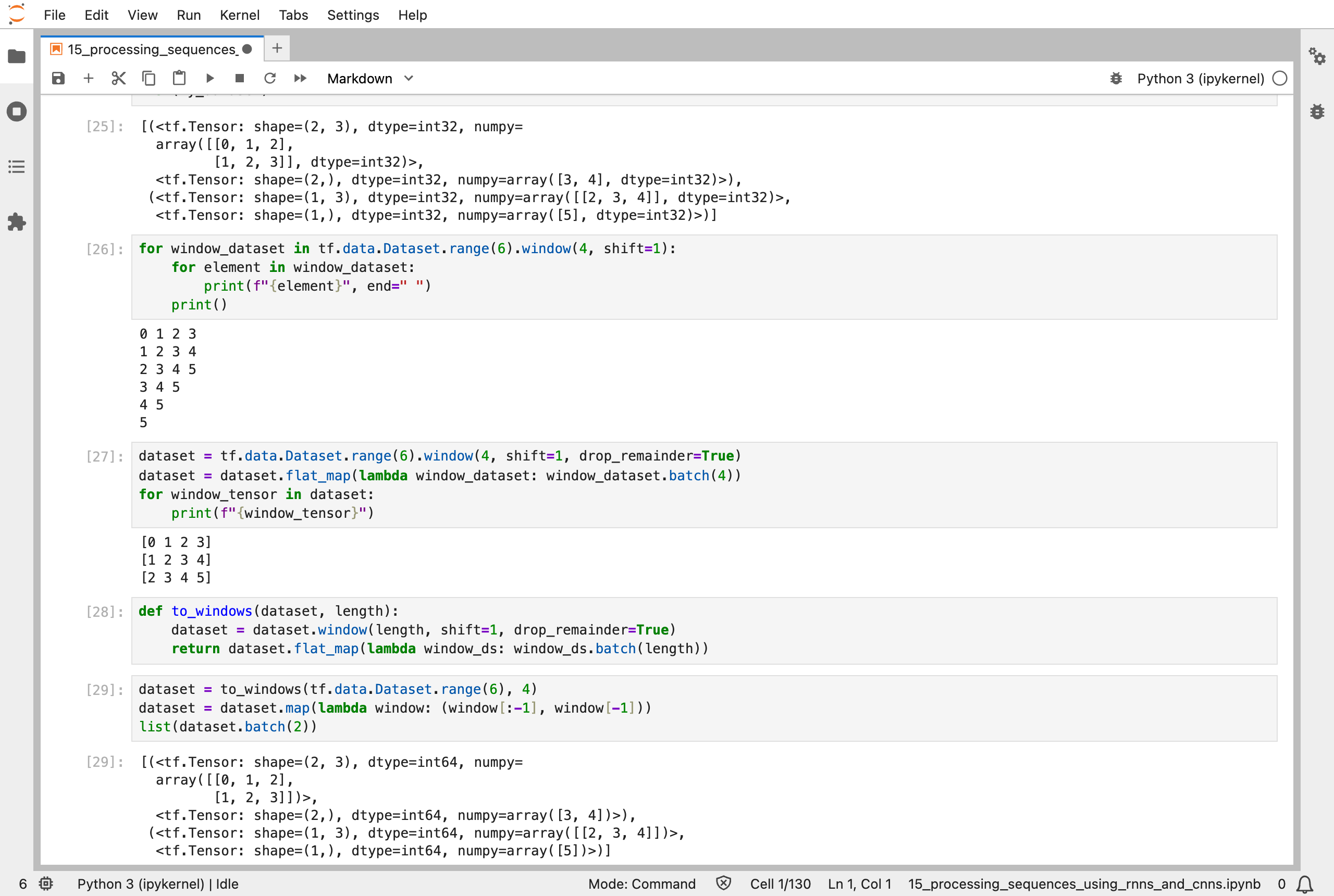
Windows of 4 over the numbers 0 to 5: each window moves one step along, and then each window is split into inputs, three numbers, and a target, the fourth
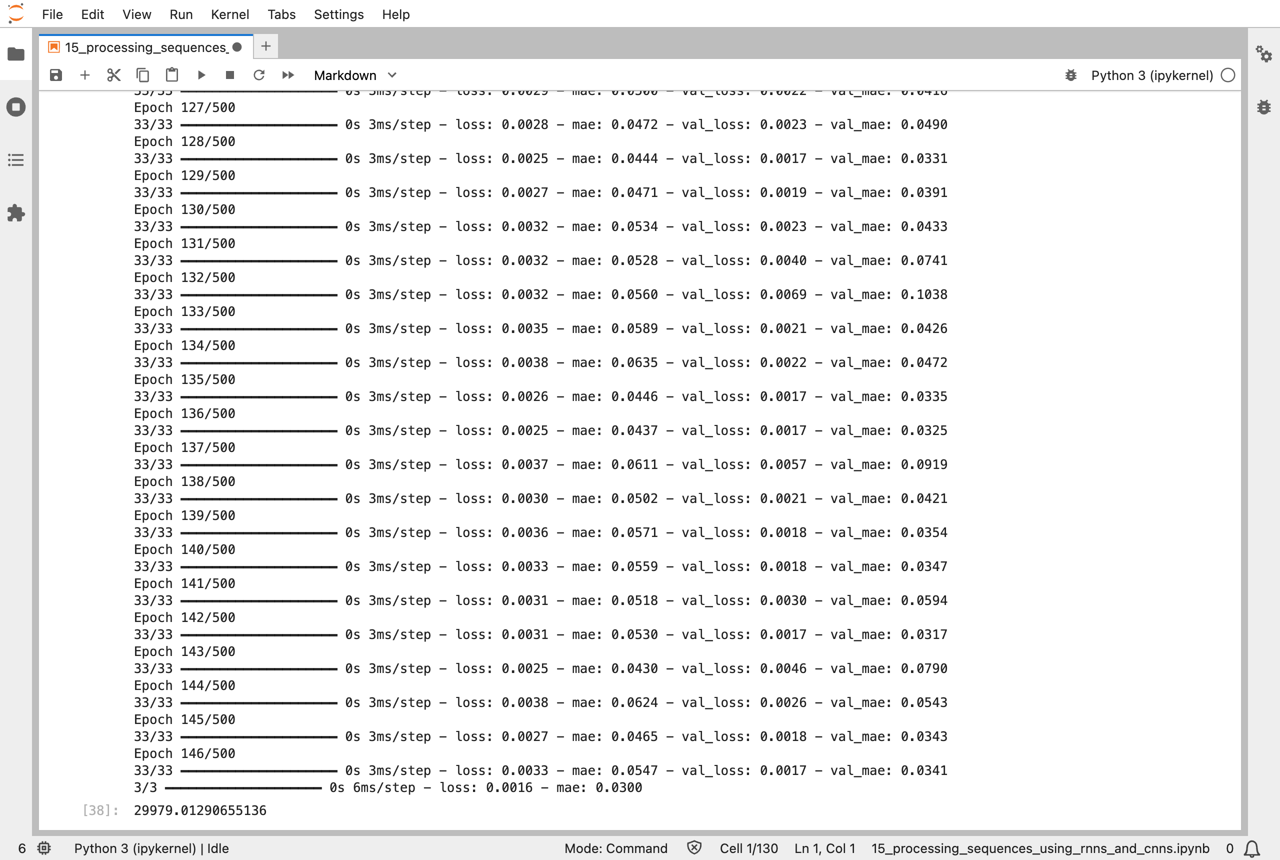
Training the 32-neuron SimpleRNN: it stopped at epoch 146, as the validation error stopped improving, with an average error of 29,979 boardings
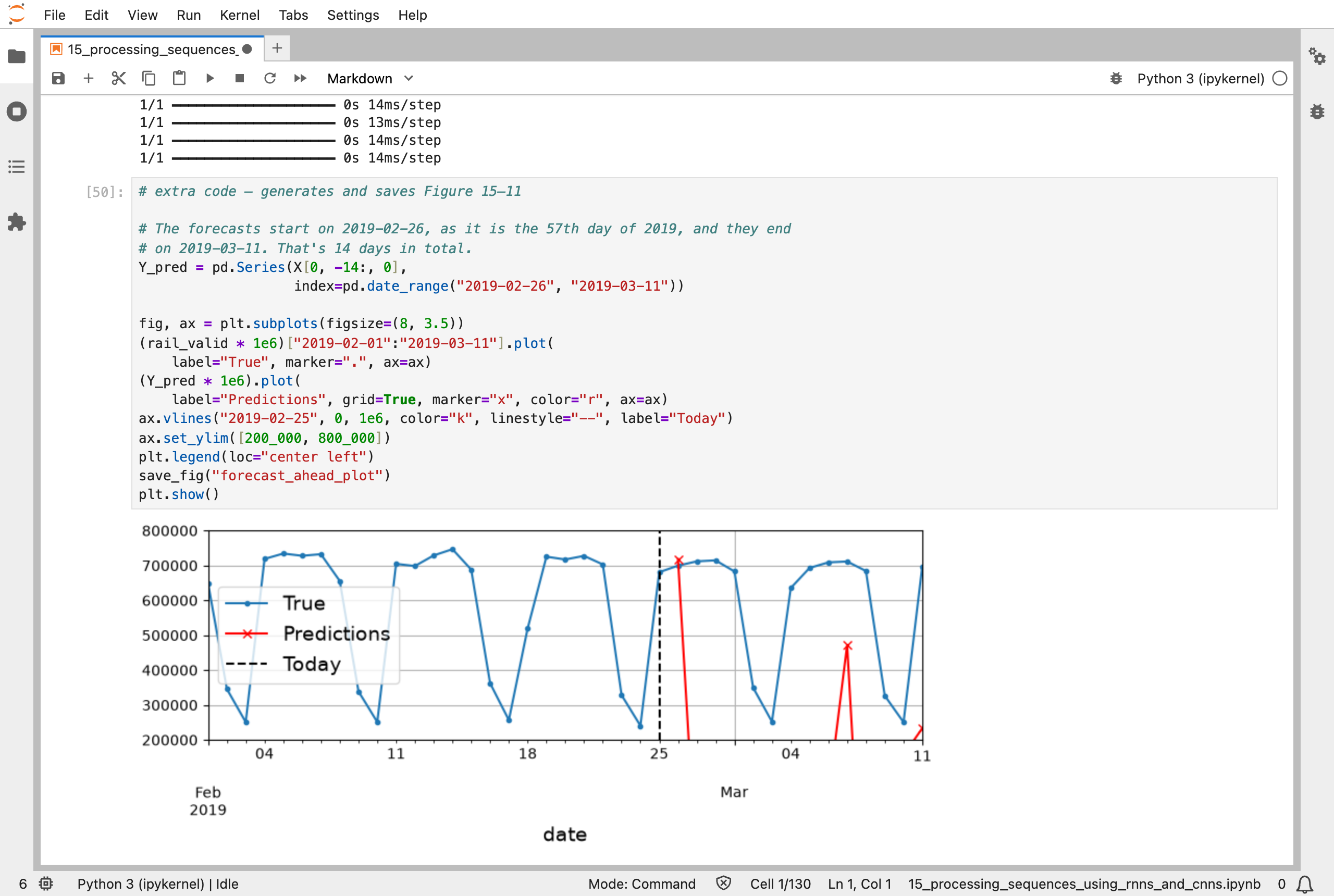
Forecasting 14 days by feeding each forecast back in: the first forecast is fine, but the next ones fall far away from the true values, and the later ones drop off the bottom of the plot
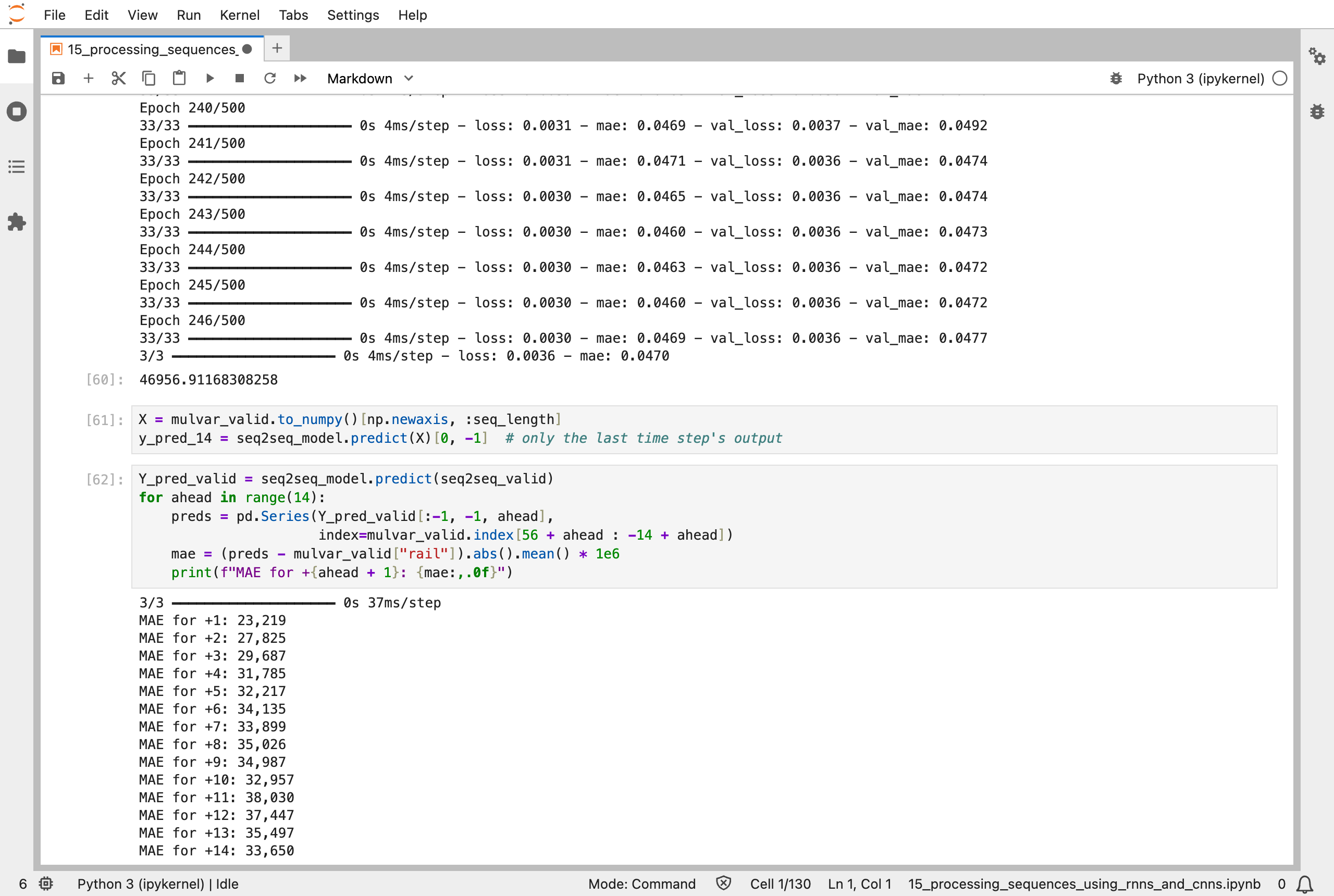
A model that forecasts all 14 days at once: the error is 23,219 for tomorrow and grows slowly, to about 33,650 for the day 14 days ahead
Next, Scikit-Learn (Part 16) works through chapter 16: natural language processing with RNNs and attention.