Scikit-Learn (Part 14)
Neil Haddley • October 13, 2026
Deep computer vision with convolutional neural networks (CNNs): filters that slide across an image, pooling, a CNN for clothing, a pretrained ResNet, and transfer learning for flowers
In Part 13, I built pipelines that feed data to a model, including images. This chapter of the Hands-On Machine Learning book is about the models that suit pictures best. Instead of looking at all the pixels at once, as the network in Part 10 did, they look at small patches, with the same few numbers reused across the whole picture. They are called convolutional neural networks (CNNs).
The tasks are real. A small CNN looked at the same clothing pictures as Part 10 and was right on 90.5% of the test pictures, about three points better than the earlier network. And an existing network, trained by someone else on a million pictures, was retrained a little to tell five kinds of flowers apart, reaching 91.8% on pictures that it had not seen, though it had memorised its training pictures almost perfectly (99.9%).
Key Points
The lesson: a picture has the same patterns wherever they are, such as an edge or a corner. A convolutional layer slides a small grid of numbers, a filter, across the whole picture, so it finds a pattern wherever it appears and needs far fewer numbers than a layer connected to every pixel. Training nudges the filters: they start random, and become edge finders, then texture finders, then finders of parts of objects. And because someone else's network has already learned those, starting from it beats starting from nothing.
What I learned from it:
- Shrinking the picture between layers, by keeping only the strongest value in each small region, widens what each later layer sees.
- Reusing a trained network works in two steps: first train only the new top layers, then unfreeze part of the old network and keep training with a smaller step size.
- A network can learn its training pictures almost perfectly and still be worse on new ones, as the flower network shows.
The chapter also covers the famous network designs of the last 30 years, and finding where in a picture an object is. I do not go into those here.
Quick Example
A small CNN for the same Fashion MNIST clothing pictures as Part 10: five convolutional layers with pooling between them, then three ordinary layers at the end.
PYTHON
1DefaultConv2D = partial(tf.keras.layers.Conv2D, kernel_size=3, padding="same",
2                        activation="relu", kernel_initializer="he_normal")
3model = tf.keras.Sequential([
4    DefaultConv2D(filters=64, kernel_size=7, input_shape=[28, 28, 1]),
5    tf.keras.layers.MaxPool2D(),
6    DefaultConv2D(filters=128),
7    DefaultConv2D(filters=128),
8    tf.keras.layers.MaxPool2D(),
9    DefaultConv2D(filters=256),
10    DefaultConv2D(filters=256),
11    tf.keras.layers.MaxPool2D(),
12    tf.keras.layers.Flatten(),
13    tf.keras.layers.Dense(units=128, activation="relu", kernel_initializer="he_normal"),
14    tf.keras.layers.Dropout(0.5),
15    tf.keras.layers.Dense(units=64, activation="relu", kernel_initializer="he_normal"),
16    tf.keras.layers.Dropout(0.5),
17    tf.keras.layers.Dense(units=10, activation="softmax")
18])
Each Conv2D layer slides its filters across the picture, and each MaxPool2D halves its width and height. The network has 1,413,834 numbers, and these are the results from my run, after 10 passes through 55,000 pictures:
| Measure | Result |
|---|---|
| Training pictures right, in the last pass | 92.9% |
| Validation pictures right, in the last pass | 90.9% |
| Test pictures right | 90.5% |
| The dense network from Part 10: 266,610 numbers, after 30 passes | 87.4% of the test pictures right |
The CNN has more numbers than the network from Part 10, not fewer, because it is deeper and has a wide final layer. But it learned faster, after only 10 passes, and got about 3 percentage points more of the test pictures right. Each pass took about 80 seconds.
And here is what I got when I took a ResNet50 that someone else had trained on ImageNet, and asked it about the two sample photos that come with Scikit-Learn:
| Photo | Its three best guesses |
|---|---|
| A temple building by a lake | palace 54.69%, monastery 24.71%, bell cote 18.55% |
| A close-up of a flower | vase 32.67%, daisy 17.82%, honeycomb 12.04% |
The first answer is reasonable. The second is a reminder that the model has 1,000 categories to choose from, and none of them is the right one for a plain close-up of this flower.
What training means here
Nothing about learning changes here either. The numbers in the filters are nudged exactly as in Part 10 and Part 11: a batch of pictures goes in, the loss is measured, backpropagation finds the slopes, and every number moves a little. A filter is not designed by a person. It starts random, and training makes it useful.
The notebook shows this by comparing two kinds of filter. First, two filters made by hand, one a vertical line of ones and one a horizontal line. Applied to a photo, the first keeps the vertical edges, such as the pillars of a building, and the second keeps the horizontal ones. Second, filters that start out random, with no training at all: even these act like edge detectors, which the book says is a useful starting point. Training then improves them, layer by layer, from edges to textures to parts of objects.
Transfer learning is the clearest case of the training thread so far. The pretrained Xception network already has millions of numbers worth keeping, trained on pictures far more varied than 3,670 flowers. The notebook first freezes all of them, and trains only the new top layers, with a large step size (a learning rate of 0.1) for 3 epochs: that gave 85.3% validation accuracy. Then it unfreezes the network from layer 56 on, and continues for 10 epochs with a step size ten times smaller (0.01): that gave 91.8% by the end. The smaller step size matters, because large nudges would wreck what the pretrained layers already know.
My MiniGPT model has no convolutions. It looks across its text with attention, which Part 16 covers. But the idea of reusing the same small set of numbers at every position is shared: a filter is applied at every position in a picture, and MiniGPT's blocks are applied at every position in a text.
Running the notebook in Jupyter
The chapter is in the notebook that goes with the book, 14_deep_computer_vision_with_cnns.ipynb. I ran everything before the exercise solutions. It took about 75 minutes on my Mac Studio, most of it training the flower classifier, and it downloaded the pretrained ResNet50 and Xception weights and the flower pictures. Then I looked through the results in JupyterLab.
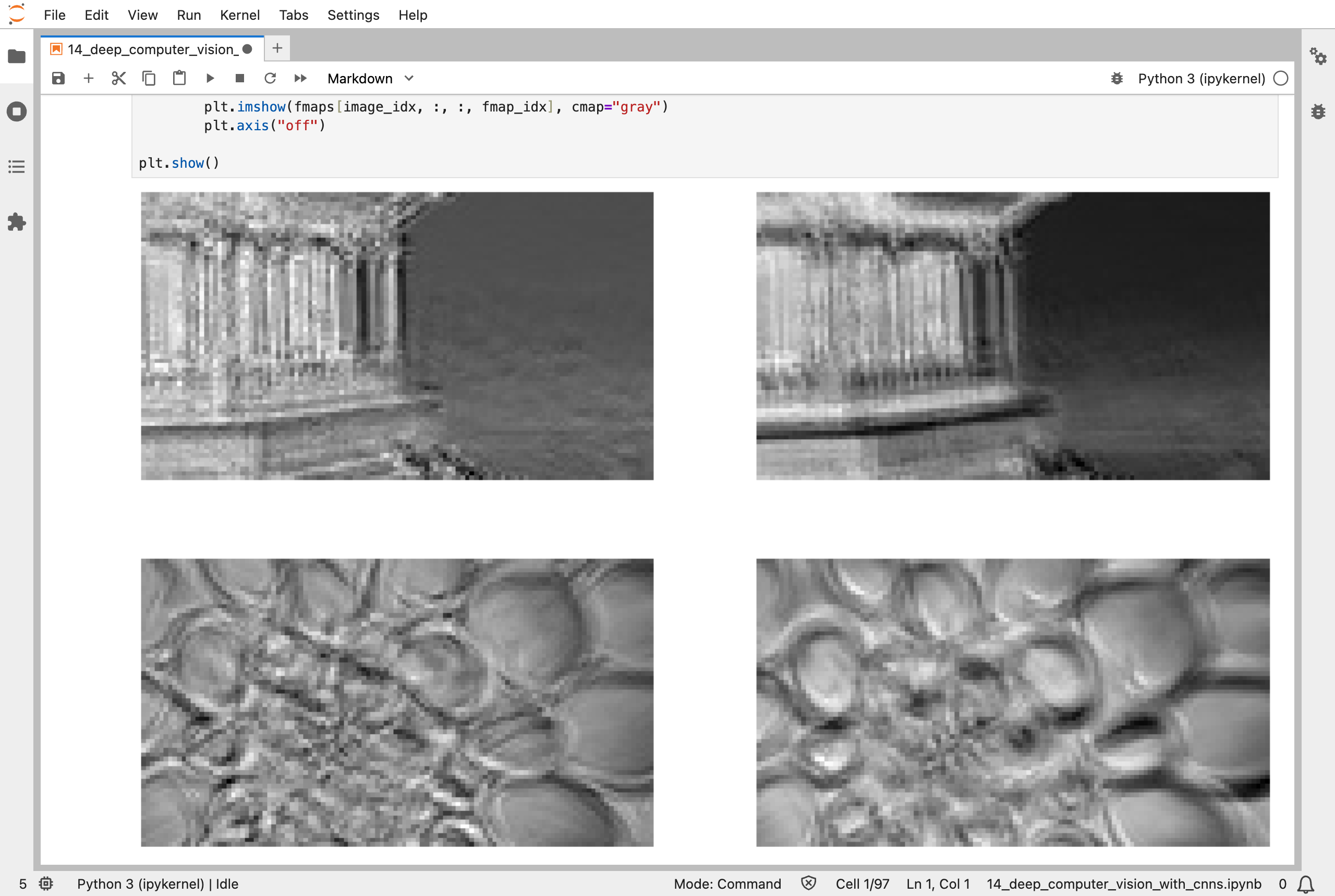
A convolutional layer with random filters, before any training: each filter gives a new grey picture of the same photo, and even these random ones pick out edges
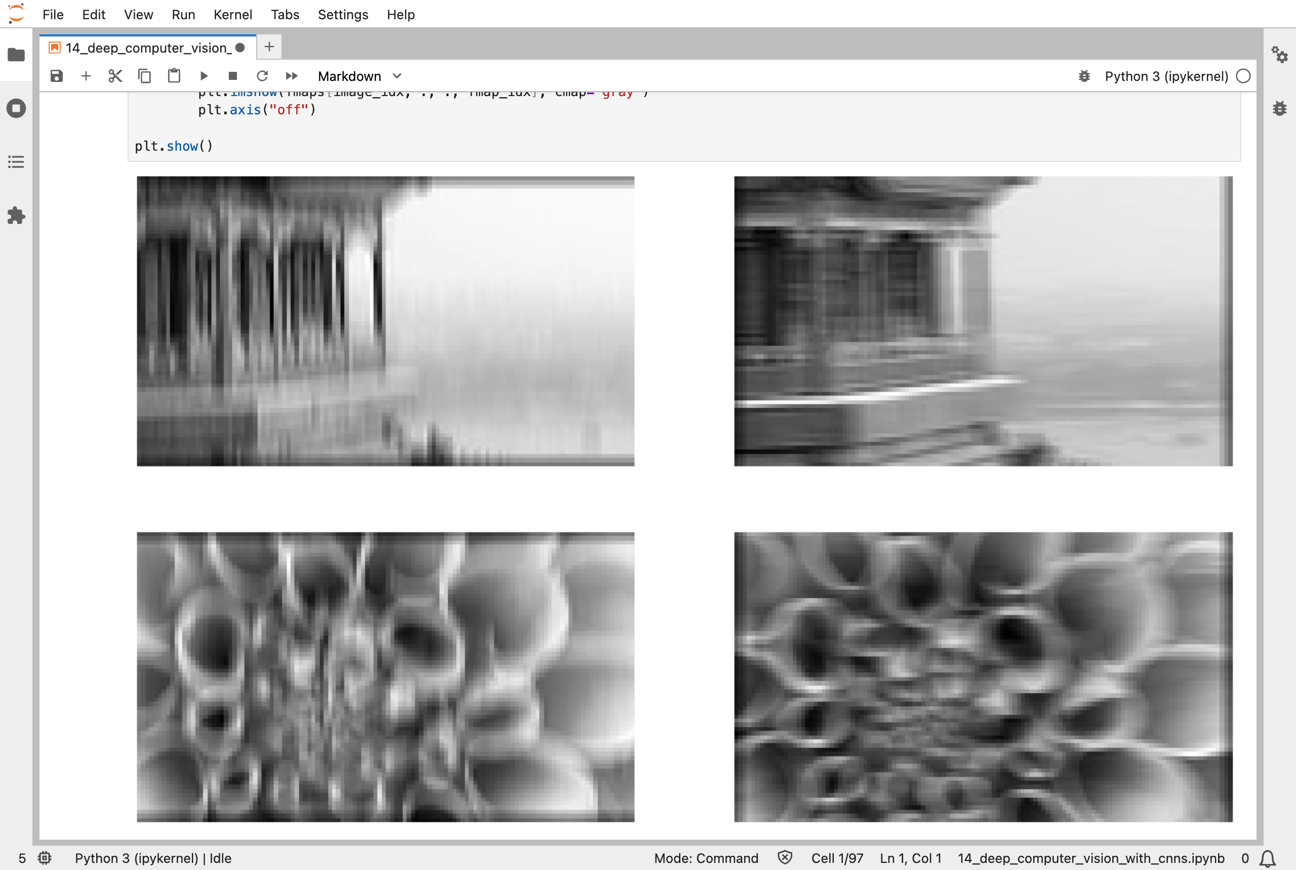
Two filters made by hand: the first, a vertical line, keeps vertical edges such as the pillars; the second, a horizontal line, keeps horizontal ones
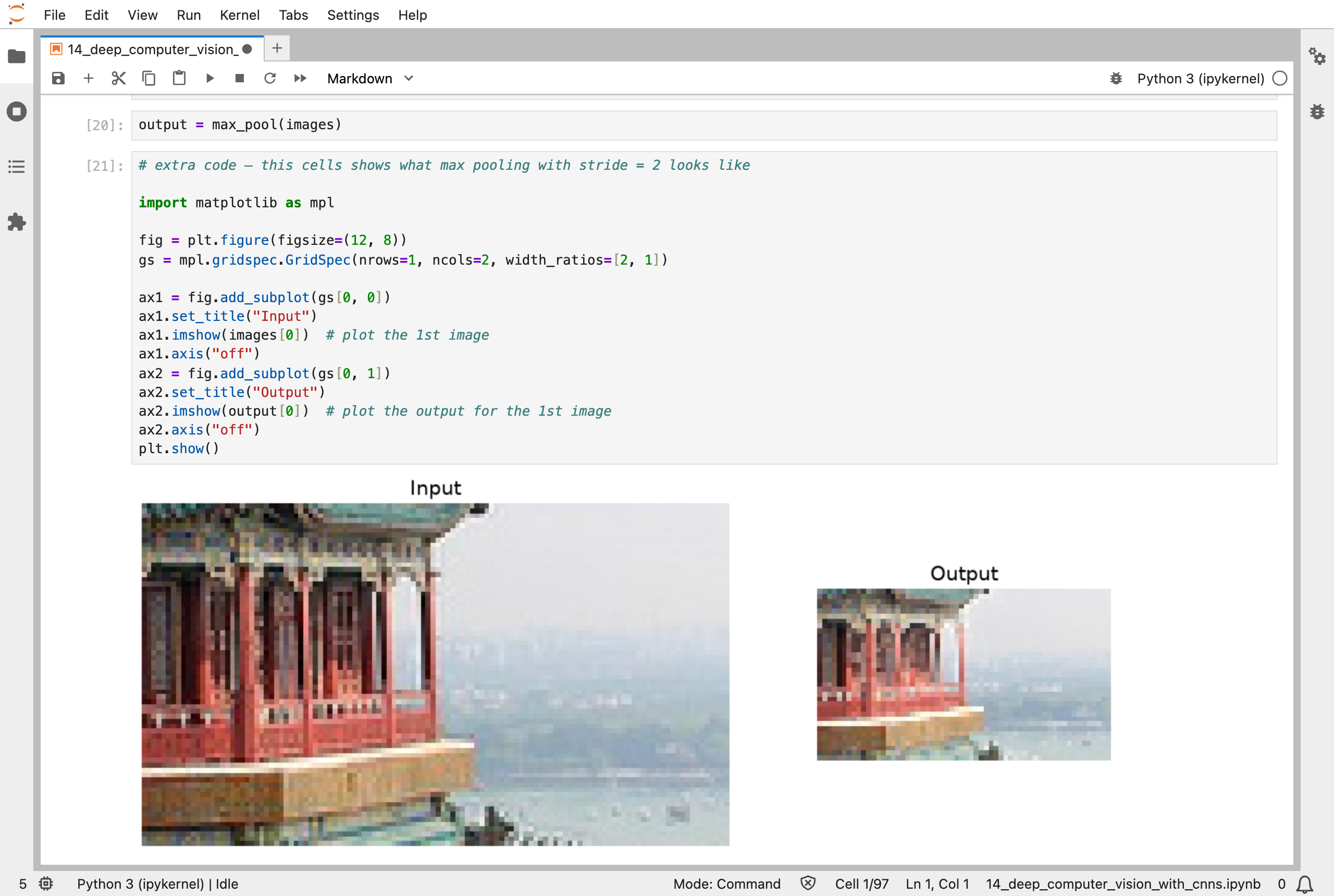
Max pooling: the output is half the width and half the height of the input, and the main shapes survive
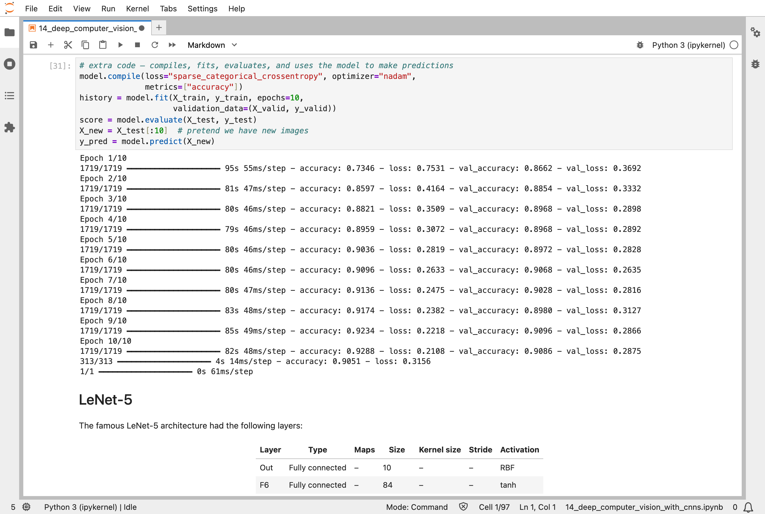
Training the CNN on Fashion MNIST: after 10 passes, 92.9% of the training pictures and 90.9% of the validation pictures are right, and 90.5% of the test pictures
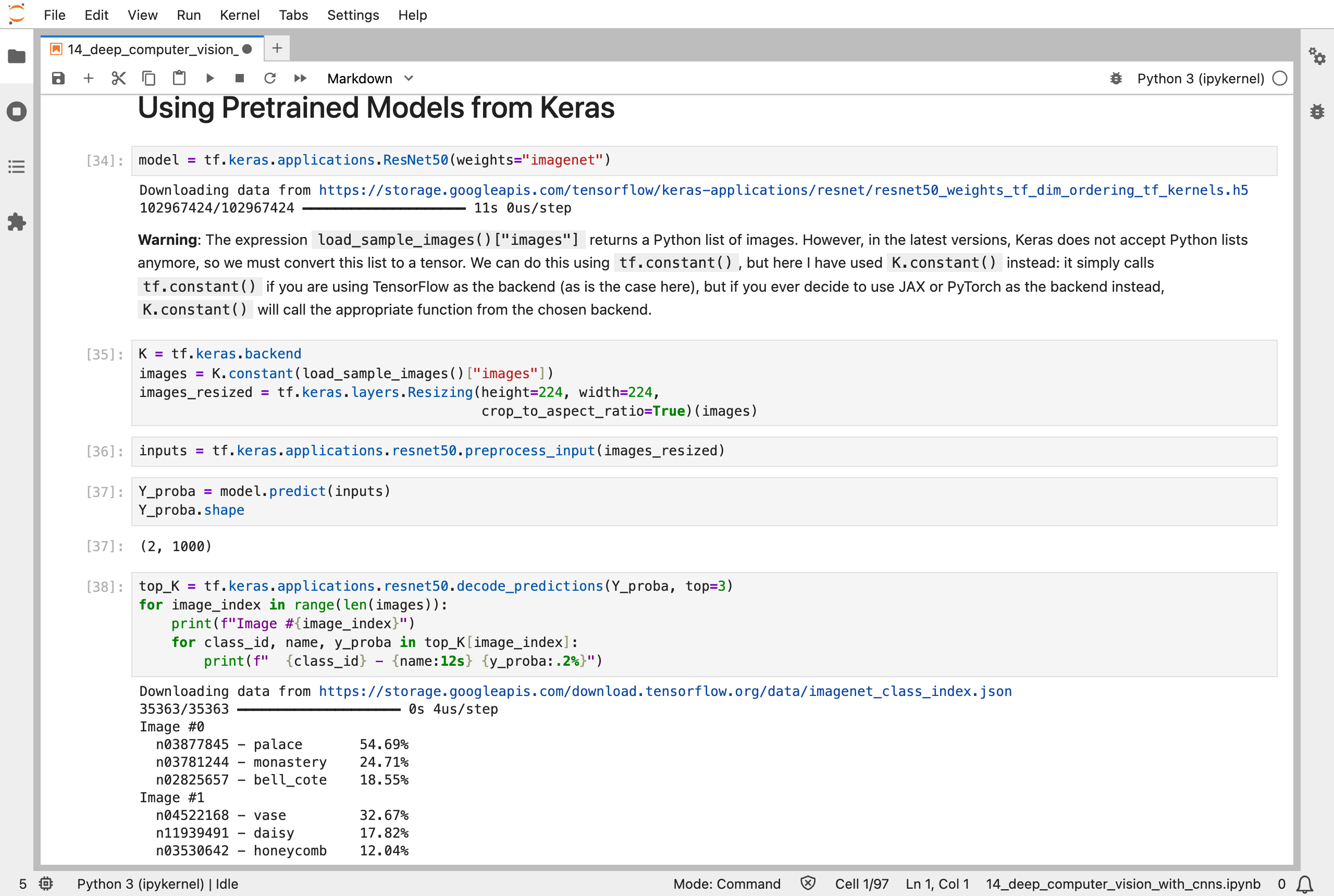
The pretrained ResNet50 on the two sample photos: it calls the building a palace, and the flower a vase
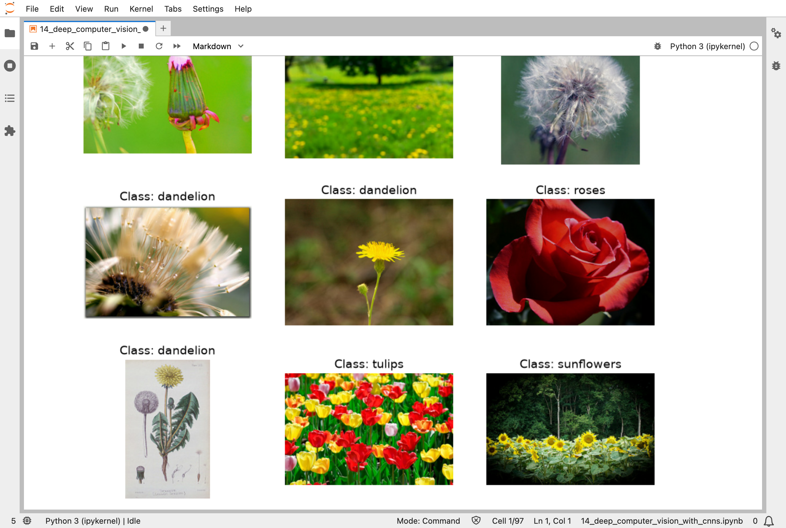
Pictures from the flower dataset, each labelled with its class: dandelions, a rose, tulips, and sunflowers
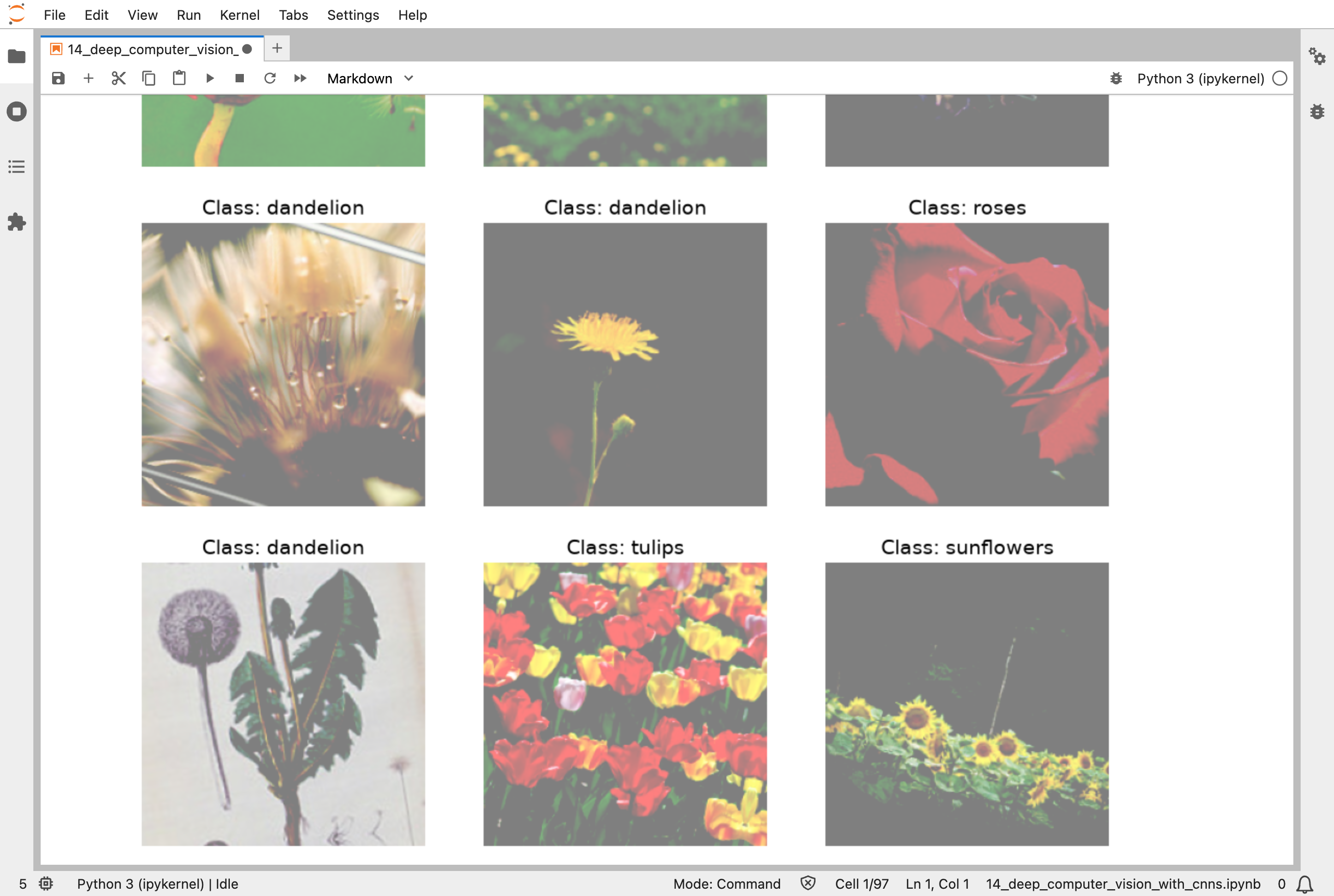
The same pictures after random flips, small rotations, and contrast changes: the notebook displays this data augmentation, but does not use it in the training that follows
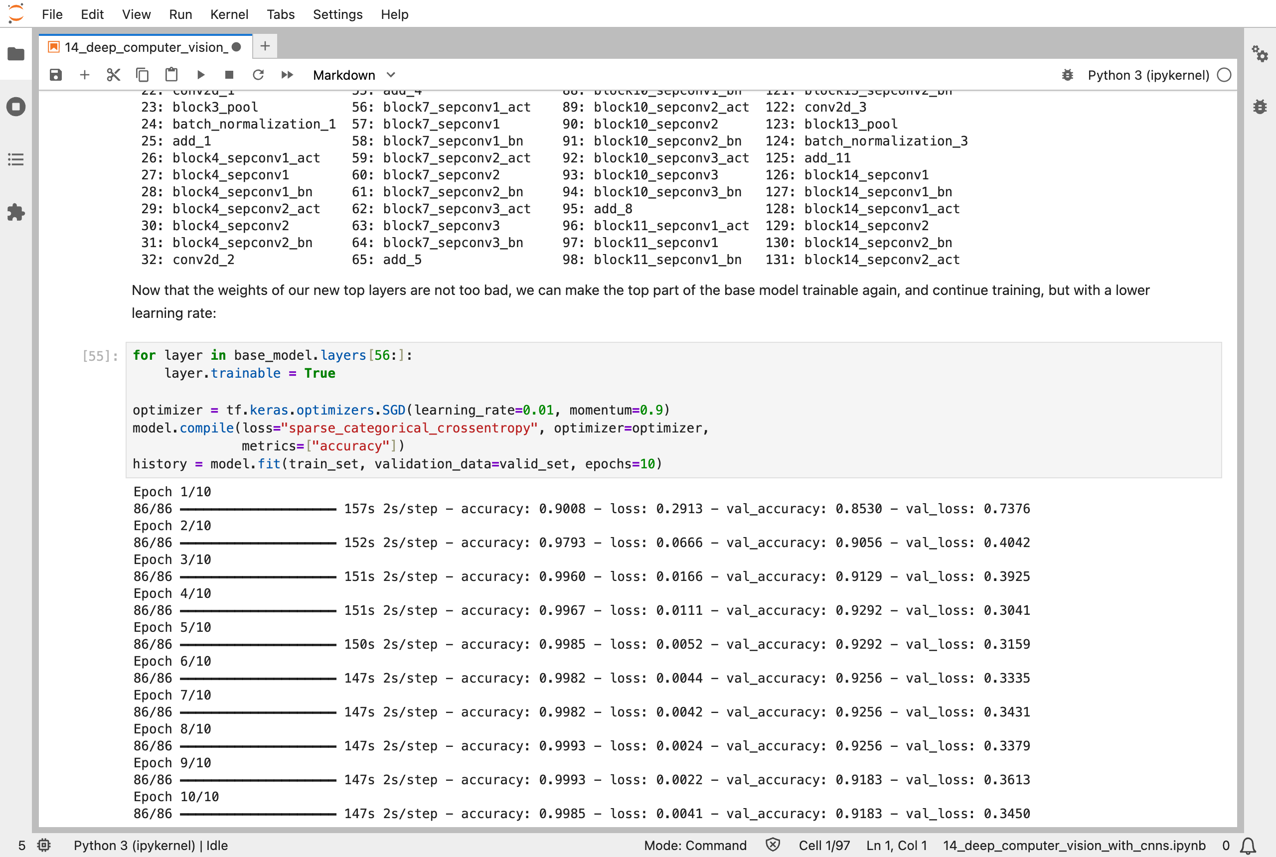
Fine-tuning the pretrained Xception: with its top layers unfrozen, the training accuracy reaches 99.9% and the validation accuracy peaks at 92.9%, then slips back to 91.8%
Next, Scikit-Learn (Part 15) works through chapter 15: processing sequences using recurrent neural networks (RNNs) and CNNs.