In Part 16, I read and generated text. This chapter of the Hands-On Machine Learning book generates pictures. The pictures are the real Fashion MNIST clothing pictures again, and the question is whether a network can learn well enough what clothing looks like to draw some that never existed. It starts with networks that squeeze a picture down to 30 numbers and rebuild it, and ends with the idea behind much of today's image generation.
In my run, a network squeezed each 784-pixel picture down to 30 numbers and rebuilt a recognisable but blurred copy. A convolutional GAN, trained for 50 passes, drew shoes, shirts, trousers, bags, and dresses that were not in the data. And a diffusion model, trained for 100 passes, drew shoes, boots, trousers, and jackets by starting from pure noise and removing it, step by step.
Key Points
The lesson: I can train a network to copy its input through a narrow middle, so that the middle becomes a compact summary of the picture. No labels are needed, because the picture is its own answer. A variation lets me throw away the first half, feed random numbers to the second half, and get new pictures. Two other ideas make better pictures. A generative adversarial network (GAN) trains a forger and a detective against each other. A diffusion model learns one very simple task, to predict the noise that was added to a picture, and repeats it many times to turn noise into a picture.
What I learned from it:
- The narrow middle is the point: a network that could pass everything through would learn nothing.
- A GAN is trained by two networks pulling against each other, and can go wrong along the way. My first plain GAN drew the same shirt shape 32 times, and recovered with longer training.
- Diffusion models are trained on a simple task and are steadier, but drawing a picture takes thousands of steps, which is why it takes much longer than training one step.
The chapter also covers many kinds of autoencoder, such as ones that remove noise, which appear in the table below.
Quick Example
An autoencoder for the Fashion MNIST clothing pictures from Part 10. An encoder squeezes each 784-pixel picture down to 30 numbers, and a decoder rebuilds the picture from those 30:
PYTHON
1stacked_encoder = tf.keras.Sequential([
2    tf.keras.layers.Flatten(),
3    tf.keras.layers.Dense(100, activation="relu"),
4    tf.keras.layers.Dense(30, activation="relu"),
5])
6stacked_decoder = tf.keras.Sequential([
7    tf.keras.layers.Dense(100, activation="relu"),
8    tf.keras.layers.Dense(28 * 28),
9    tf.keras.layers.Reshape([28, 28])
10])
11stacked_ae = tf.keras.Sequential([stacked_encoder, stacked_decoder])
12stacked_ae.compile(loss="mse", optimizer=tf.keras.optimizers.Nadam())
13history = stacked_ae.fit(X_train, X_train, epochs=20, validation_data=(X_valid, X_valid))
The inputs and the targets are the same pictures, X_train twice. The score is the mean squared error between each picture and its rebuilt copy: smaller is better. These are the validation scores from my run of the chapter's different autoencoders:
| Autoencoder | Validation error |
|---|---|
| Stacked: 784, 100, 30, 100, 784, 20 passes | 0.0135 |
| Same, with the encoder's weights reused by the decoder (tied), 10 passes | 0.0135 |
| Same, trained one layer at a time and then fine-tuned, 5 passes | 0.0146 |
| Convolutional, 10 passes | 0.0135 |
| Recurrent (LSTM), 10 passes | 0.0106 |
| Denoising, with half of the inputs dropped out, 10 passes | 0.0176 |
| Sparse, with a penalty on active neurons (L1), 10 passes | 0.0114 |
| Sparse, with a penalty using the Kullback–Leibler divergence (KL), 10 passes | 0.0095 |
They are all close, which is the first surprise: the choice of design matters less than I expected, for this data. A picture compressed to 30 numbers, about 4% of its 784 pixels, comes back recognisable but blurred, and the pictures below show it.
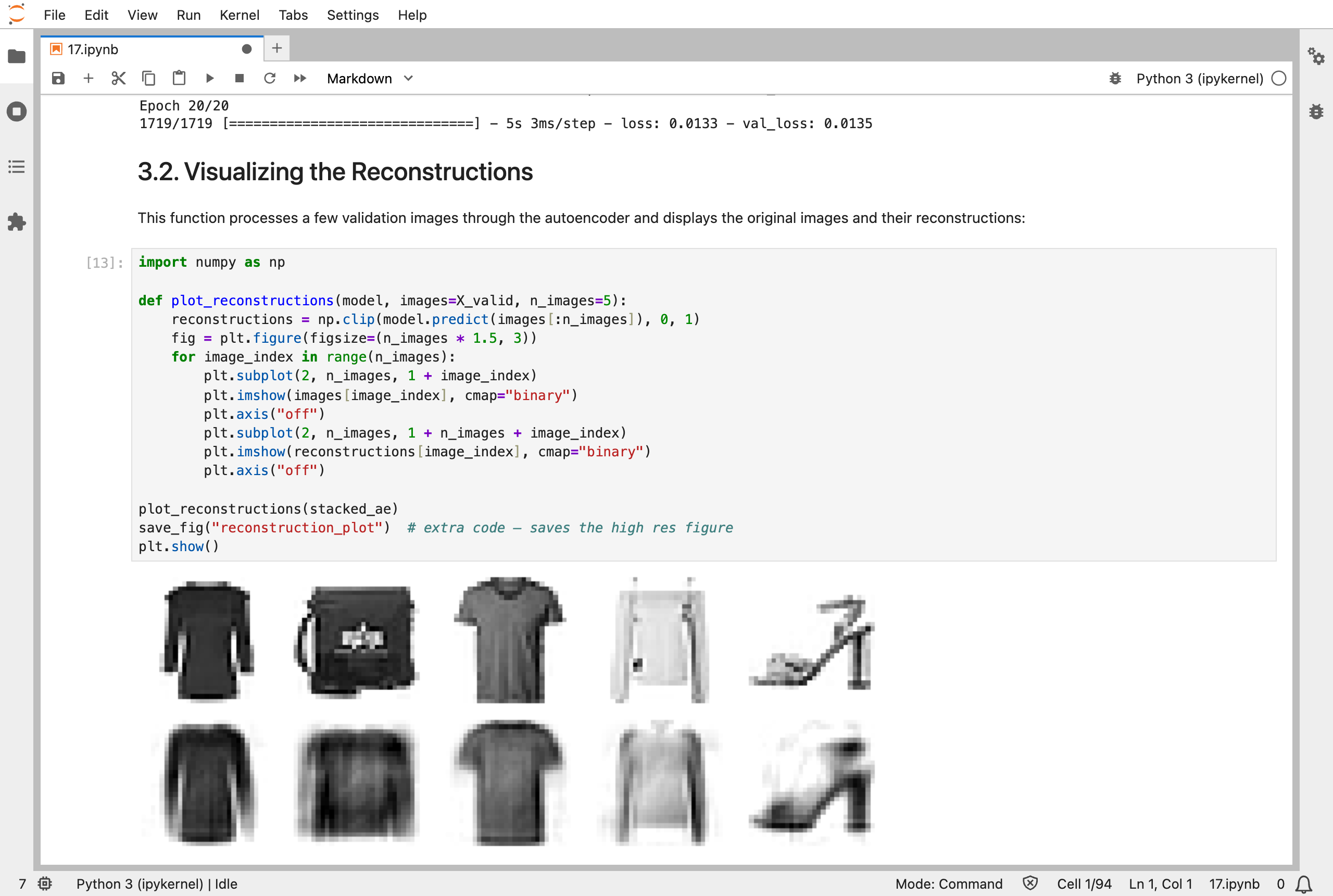
An autoencoder at work: the top row is five original pictures, and the bottom row is what the decoder rebuilt from just 30 numbers each: close, but blurred
What training means here
An autoencoder is trained as in Part 10: the loss is measured, slopes are found by backpropagation, and the numbers are nudged. What is new is the target. There are no labels: the picture is its own target, so an autoencoder can learn from any pile of pictures. Part 8 squeezed the data with principal component analysis (PCA), which is worked out directly. A linear autoencoder with no activation functions learns the same thing as PCA, by nudging, and the notebook starts there, with a small three-dimensional dataset, before adding layers.
A GAN is trained by two networks at once. In each step the discriminator is nudged to tell real pictures from generated ones, and then the generator is nudged to fool it. There is no fixed target: each network's target moves as the other improves, which is why GANs are hard to train, and why mine collapsed. A diffusion model avoids that. Its training is ordinary: the notebook adds a known amount of noise to each picture, and trains a network to predict that noise. To generate a picture, it starts from pure noise and removes a little noise, over and over, 4,000 times. That is why generating takes much longer than training one step does, a point the notebook makes.
My MiniGPT model is a generative model too: it writes text one letter at a time. A diffusion model writes a whole picture at once and sharpens it, where MiniGPT adds to its text letter by letter.
Running the notebook in Jupyter
The chapter is in the notebook that goes with the book, 17_autoencoders_gans_and_diffusion_models.ipynb. I ran everything before the final extra section, but with the three most expensive trainings cut down at first. I then ran the two GANs again at the notebook's full 50 epochs, and the diffusion model at its full 100, which took several hours on the processor. Everything else, including the autoencoders, ran as written. I ran the parts at the same time, on my Mac Studio, which took under an hour. My first attempt hung. The notebook's setup imports scikit-learn before TensorFlow, which seemed to deadlock TensorFlow on my Mac; once I removed that import, the runs finished.
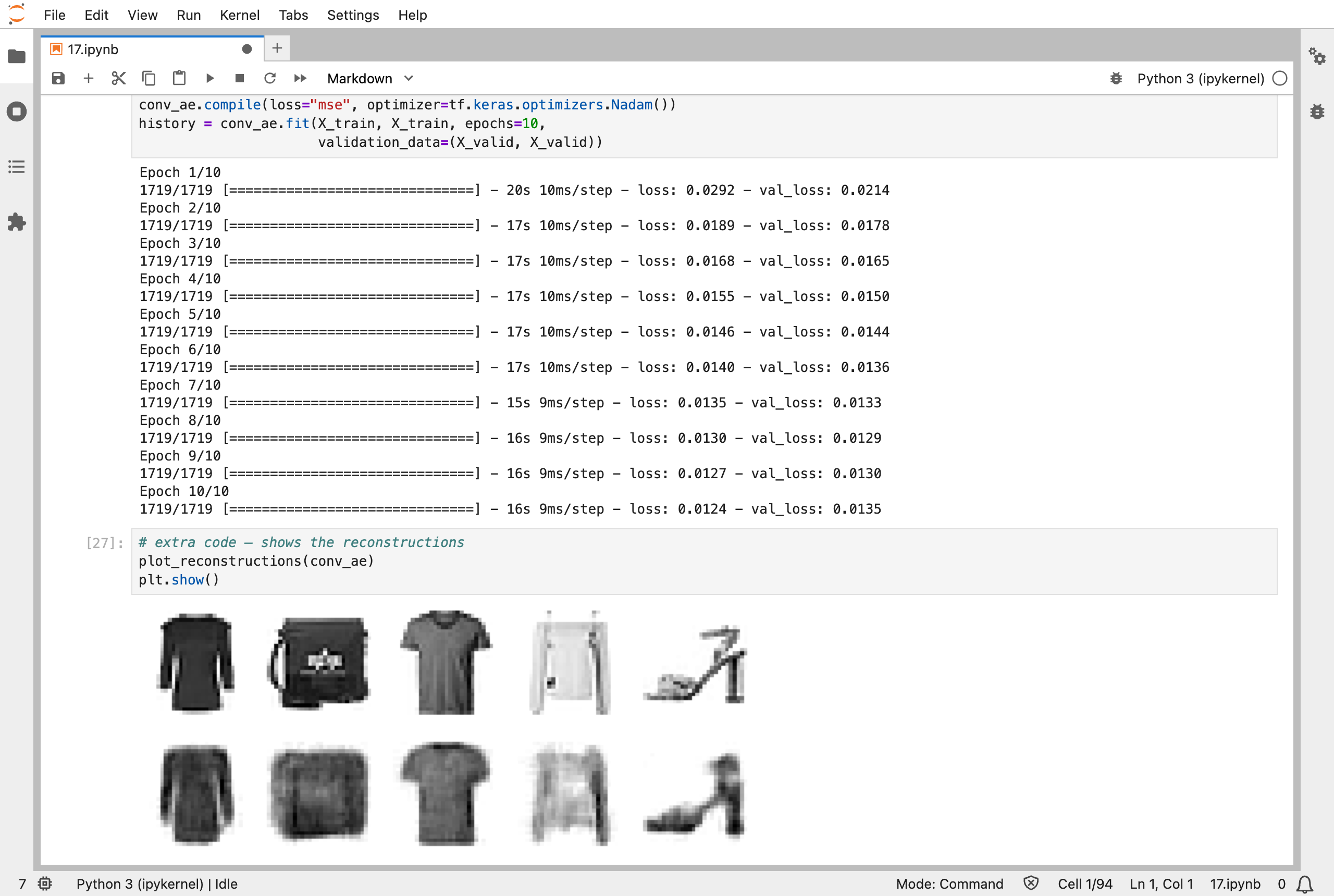
A convolutional autoencoder after 10 passes: the validation error is 0.0135, and the rebuilt pictures, bottom row, are again blurred versions of the originals above
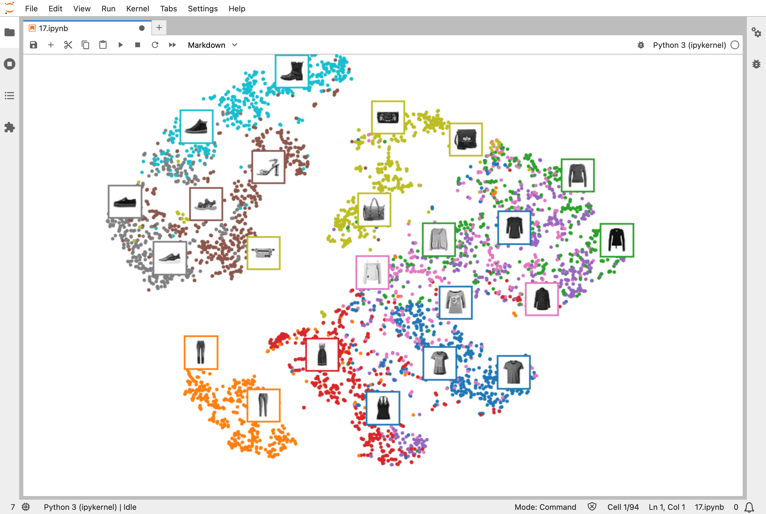
The 30 numbers for 5,000 pictures, drawn in 2D with t-SNE: shoes, bags, trousers, and tops form their own groups, though a network that never saw a label found them
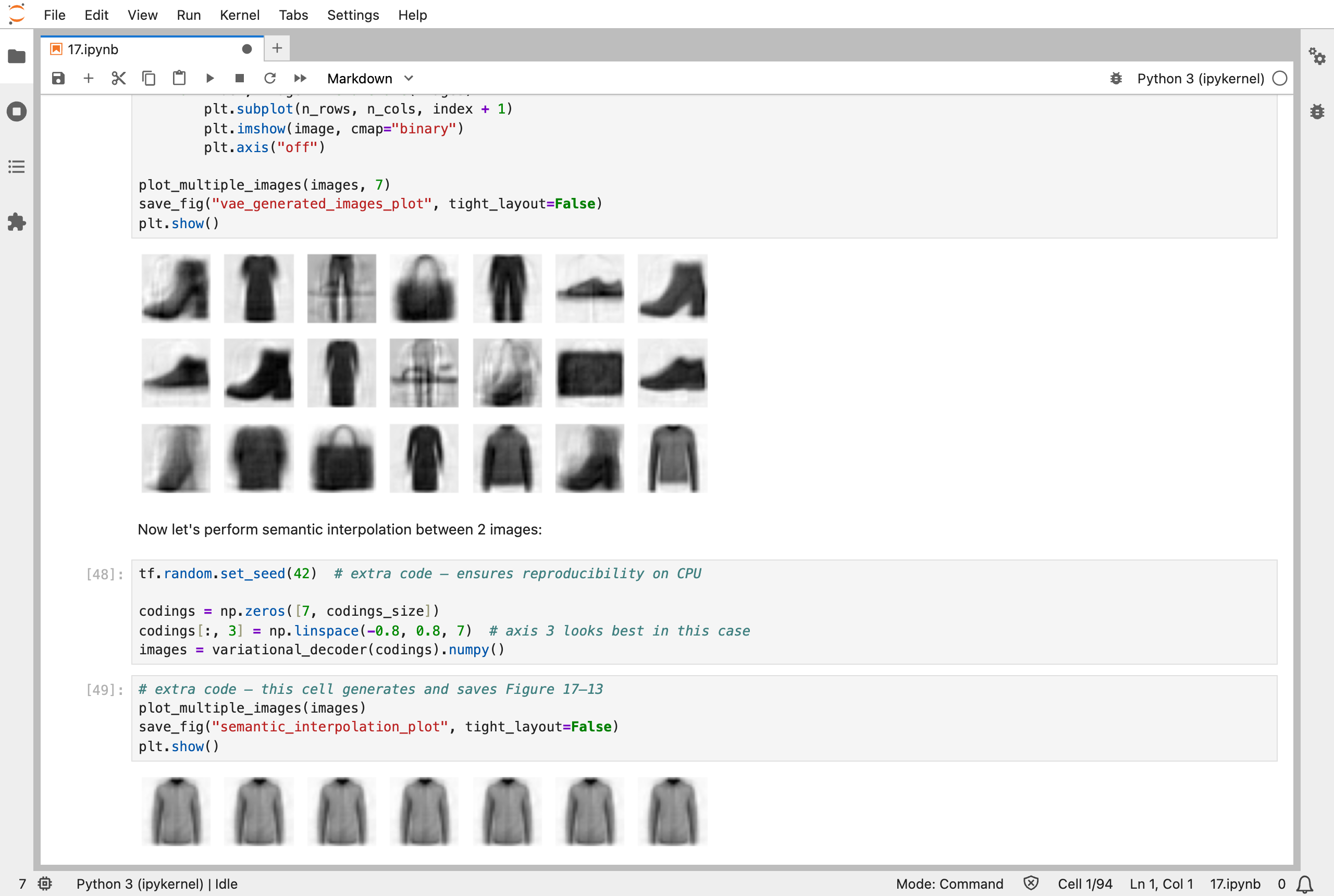
A variational autoencoder: pictures from 21 random sets of 10 numbers, and below, one picture's numbers moved a little at a time along one axis
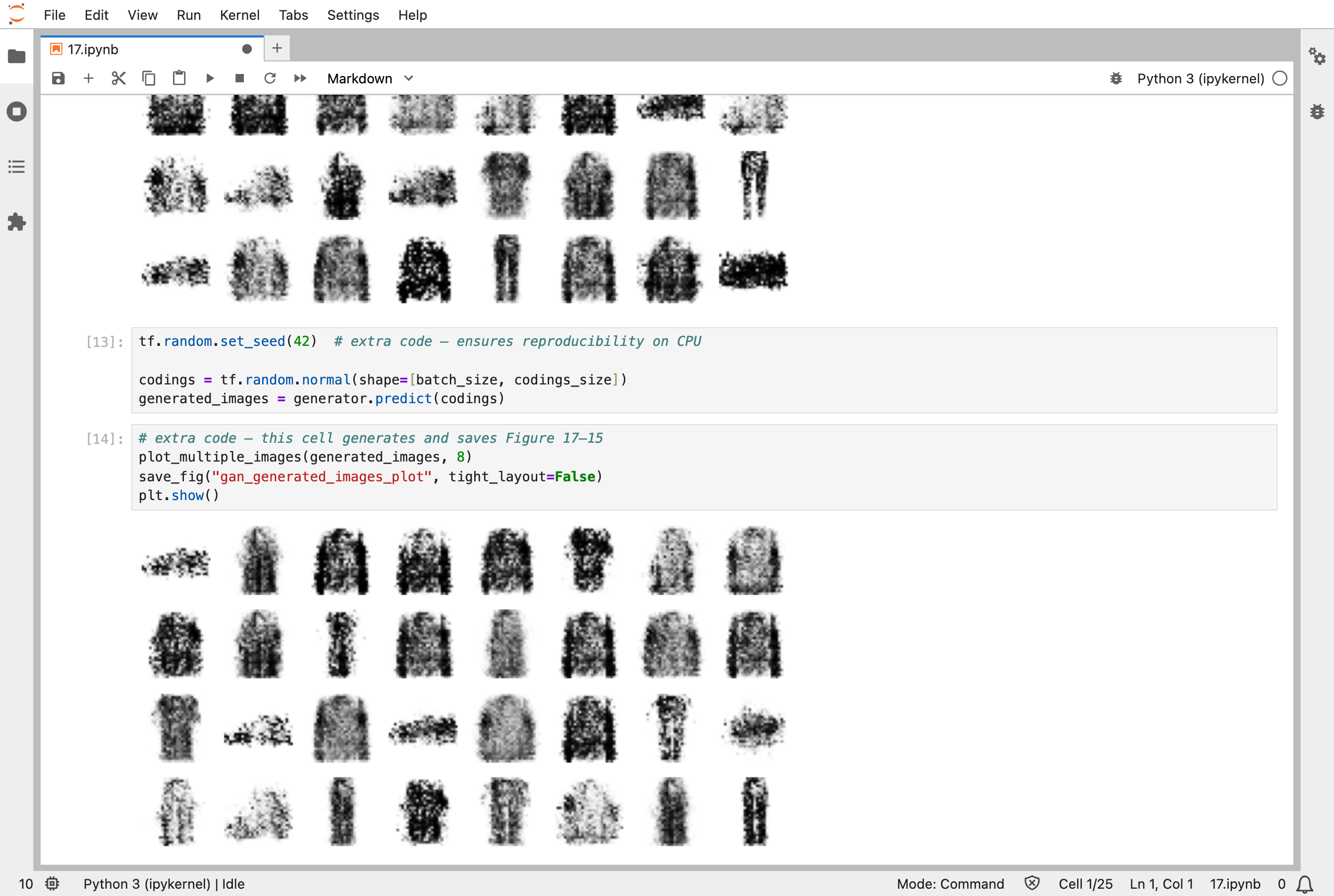
The plain GAN after 50 epochs: 32 different pictures, shirts, trousers, and shoes, but speckled with noise (after only 10 epochs it had produced the same shirt shape 32 times)
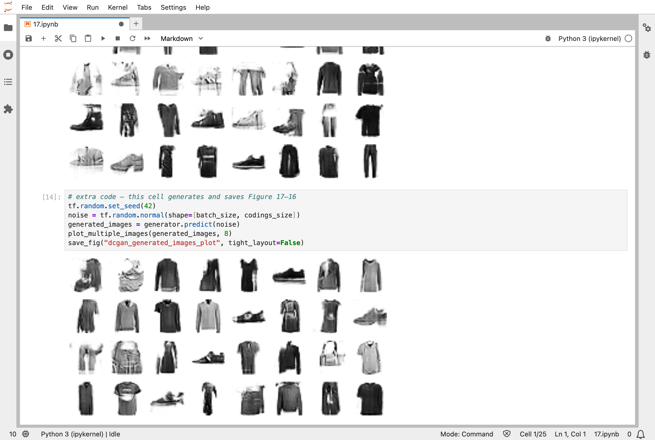
The convolutional GAN after 50 epochs: shoes, shirts, trousers, bags, and dresses, much cleaner than the plain GAN
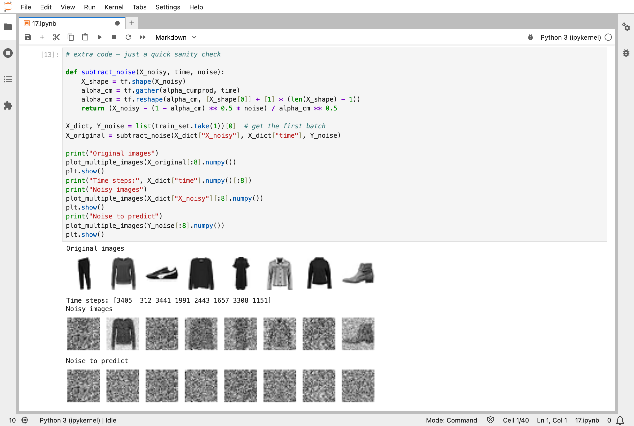
How diffusion models are trained: original pictures, the same pictures with different amounts of noise added, and the noise the network must predict
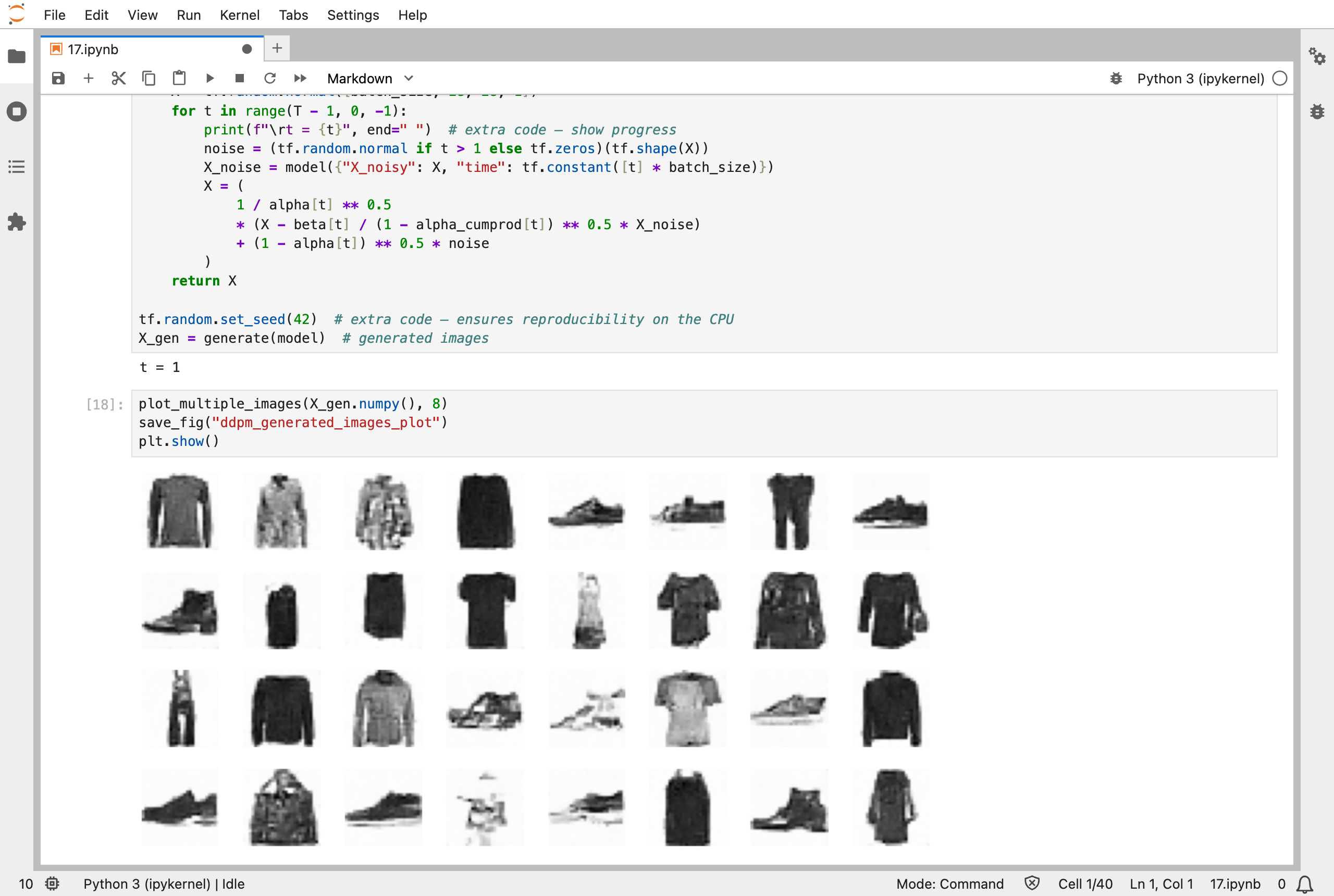
Pictures generated by the diffusion model after 100 epochs: shoes, boots, trousers, shirts, and jackets, a little blurred (after only 10 epochs they were dark blurred shapes)
Next, Scikit-Learn (Part 18) works through chapter 18: reinforcement learning.