In Part 7, I combined many models into one. This chapter of the Hands-On Machine Learning book goes the other way and shrinks the data. Each handwritten digit from Part 3 is 784 numbers, one for each pixel, but most of them tell a model very little: the pixels in the corners are almost always blank. The problem is real, and the digits are the same real ones. The question is how few numbers can still describe an image.
The answer was 154. A method called principal component analysis (PCA) finds the directions in which the images differ most, and keeps only those. With 154 numbers for each image instead of 784, I kept 95% of the variation between images, and could rebuild a recognisable digit from them, a little blurred.
Key Points
The lesson: most of a picture's numbers are redundant, and a few well-chosen ones keep nearly everything. Squeezing the data like this throws some information away, so it is there to make training faster, or to let a person see the data, and not to make a model better.
What I learned from it:
- 154 well-chosen numbers keep 95% of the variation in an image's 784.
- Flattening data that lies along a curve mixes up points that were far apart. Methods for curved data, such as t-SNE (t-distributed stochastic neighbor embedding), unroll it instead, so that neighbours stay together. t-SNE lays out many-numbered data in 2D so that I can see it.
- PCA is worked out directly, in one calculation. t-SNE is the one in this chapter that nudges.
The chapter also covers faster versions of PCA for very big data, and several other ways to unroll curved data, which I mention only in a screenshot.
Quick Example
PCA on the 60,000 MNIST training images, keeping just enough directions for 95% of the variance:
PYTHON
1from sklearn.decomposition import PCA
2
3pca = PCA(n_components=0.95)
4X_reduced = pca.fit_transform(X_train)
Here is what PCA found when I ran the notebook:
| Data | Before | After | Variance kept |
|---|---|---|---|
| Small 3D dataset | 3 | 2 | 91% |
| MNIST digits | 784 | 154 | 95% |
"Before" and "After" are the number of dimensions. For the 3D dataset, the first direction keeps 76% of the variance and the second 15%.
The chapter also searches for the best number of dimensions to feed a classifier, on 1,000 of the images: 23 for a random forest, and 67 for an SGDClassifier.
What training means here
PCA does not nudge, and it does not need to. Its directions come from a direct calculation, so fit simply works them out, much like the straight line in Part 1. There are faster versions for very big data, which get close to the same answer.
Another method, random projection, learns nothing at all: it multiplies the data by a random table of numbers, and the number of dimensions to keep comes from a formula, not from the data.
t-SNE is the one that nudges. It starts by placing every point at random in 2D, then repeatedly moves them by gradient descent, so that points that were neighbours in the original space end up near each other. Unlike every model so far, what it nudges is not a set of model numbers but the positions of the points themselves. My MiniGPT model nudges its 826,433 numbers the same way, with slopes found by backpropagation.
Running the notebook in Jupyter
The chapter is in the notebook that goes with the book, 08_dimensionality_reduction.ipynb. I ran everything before the exercise solutions, which took about 7 minutes on my Mac Studio, and then looked through the results in JupyterLab.
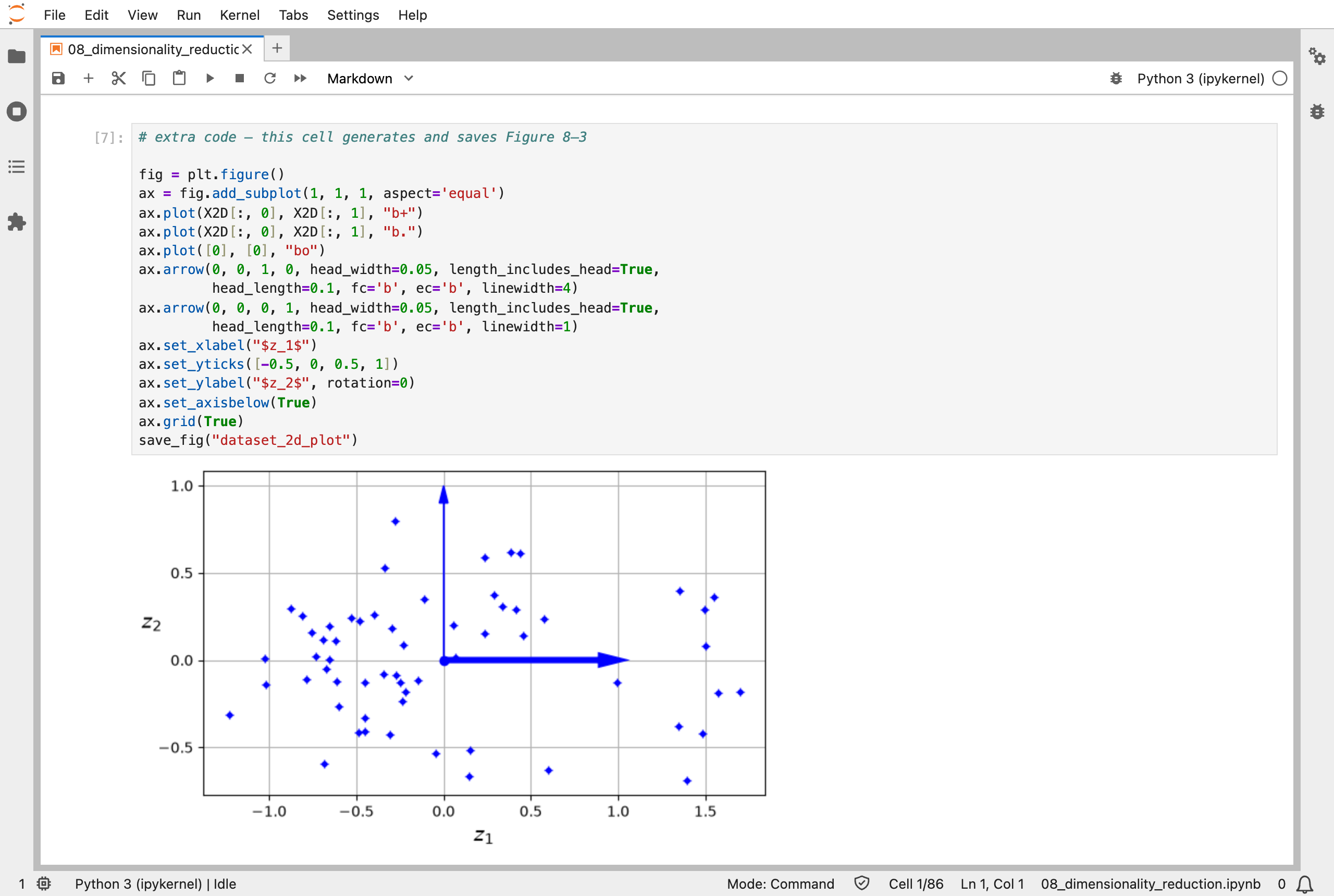
A small 3D dataset projected onto the flat surface it lies closest to: two numbers per point instead of three
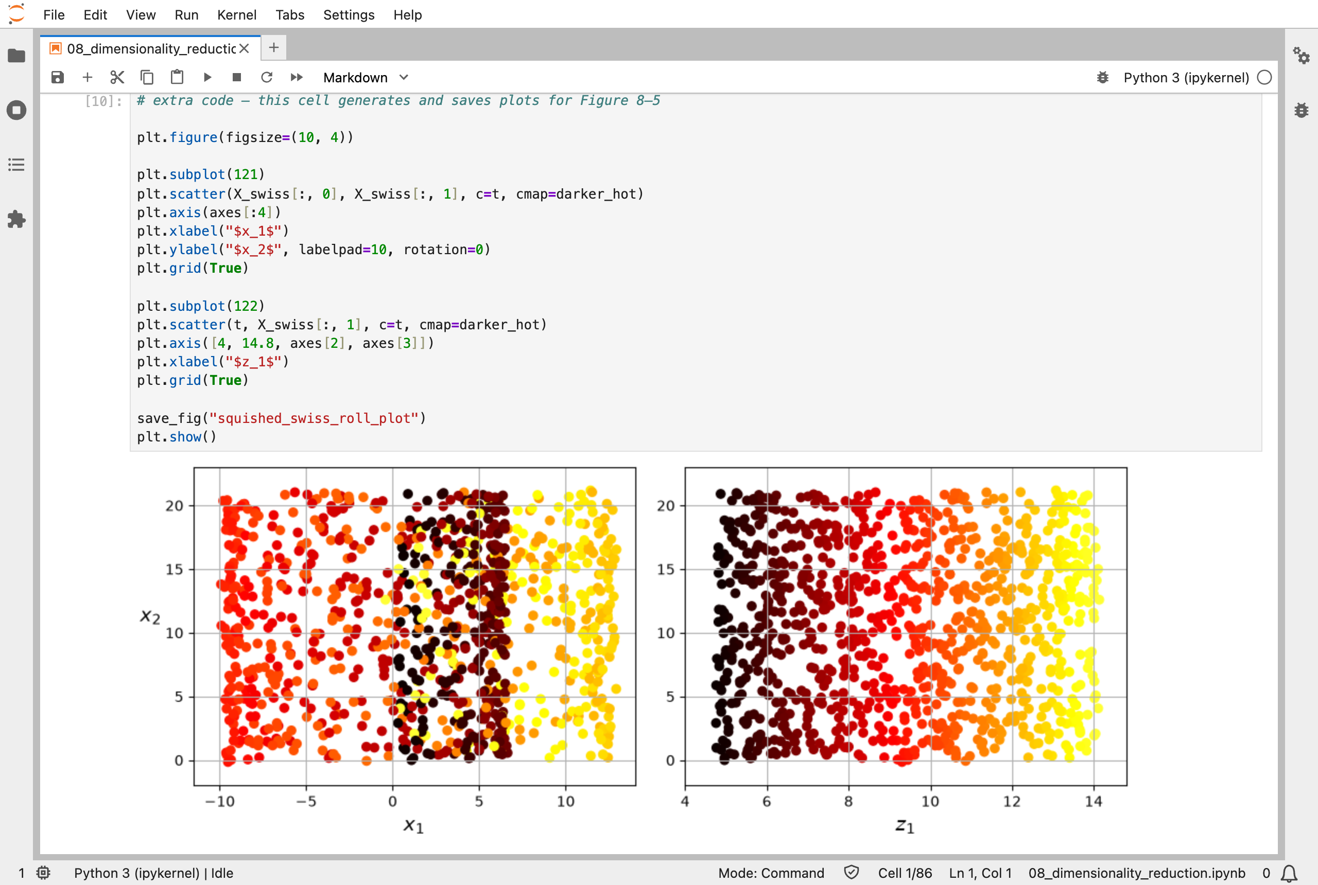
The Swiss roll: squashing it flat (left) mixes up the colours, while unrolling it (right) keeps them in order
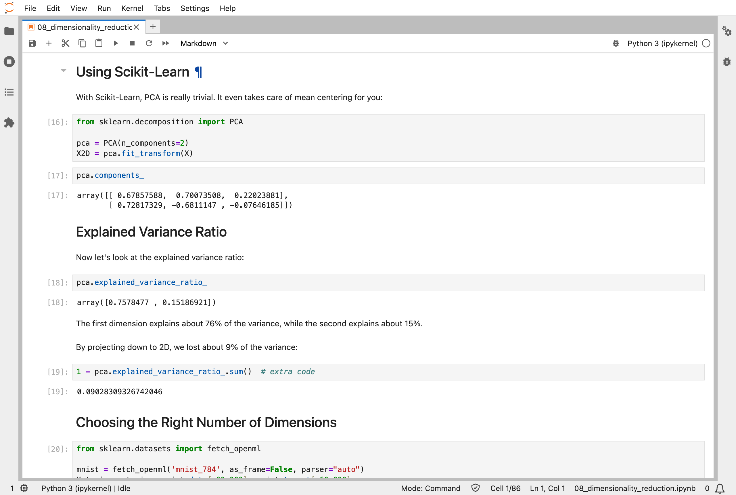
I ran PCA in two lines: the first direction keeps about 76% of the variance and the second about 15%, so going from 3D to 2D loses about 9%
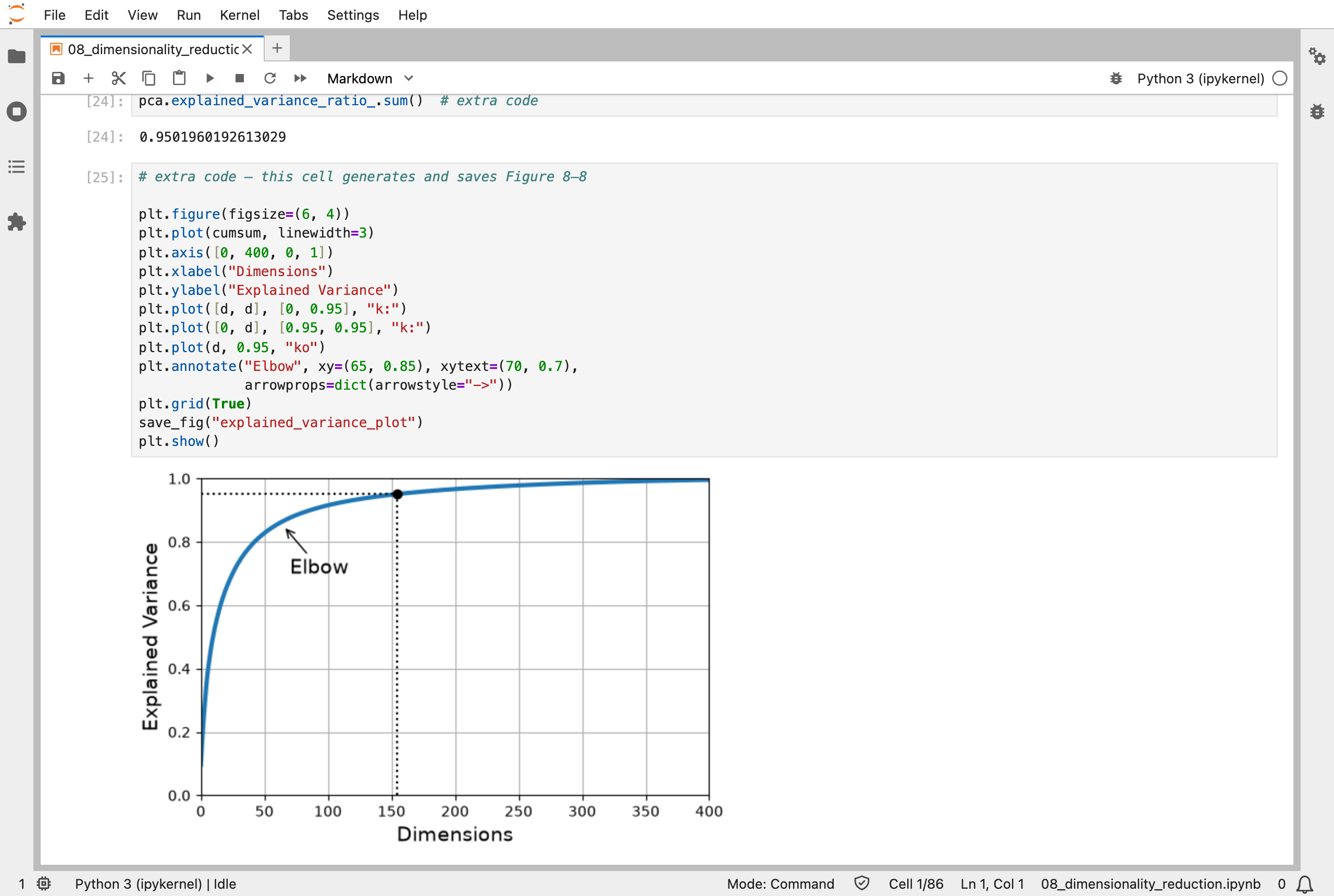
The variance kept against the number of dimensions for MNIST: it climbs fast, and 154 dimensions keep 95% of it
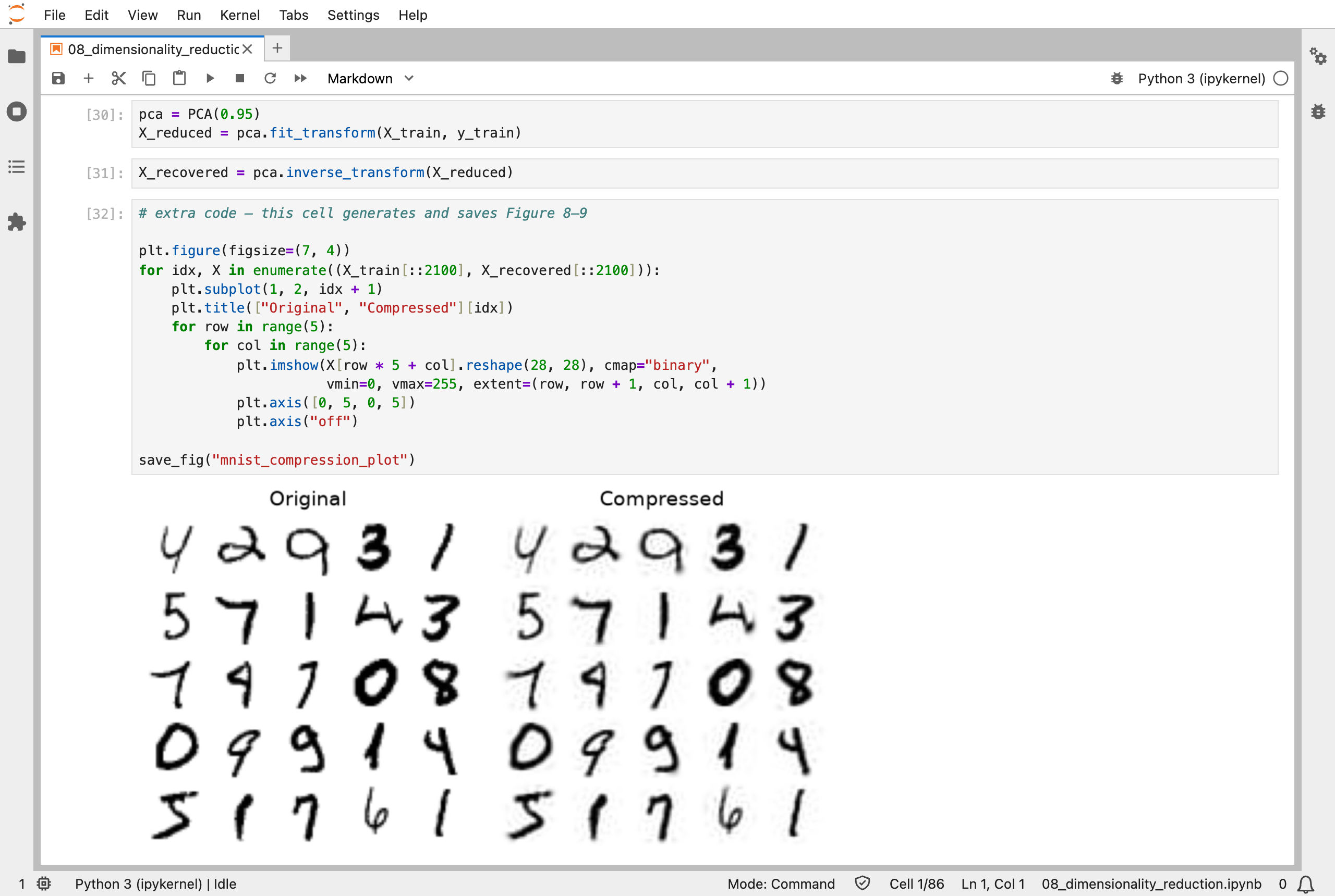
Digits rebuilt from 154 numbers instead of 784 are a little blurred, but still easy to read
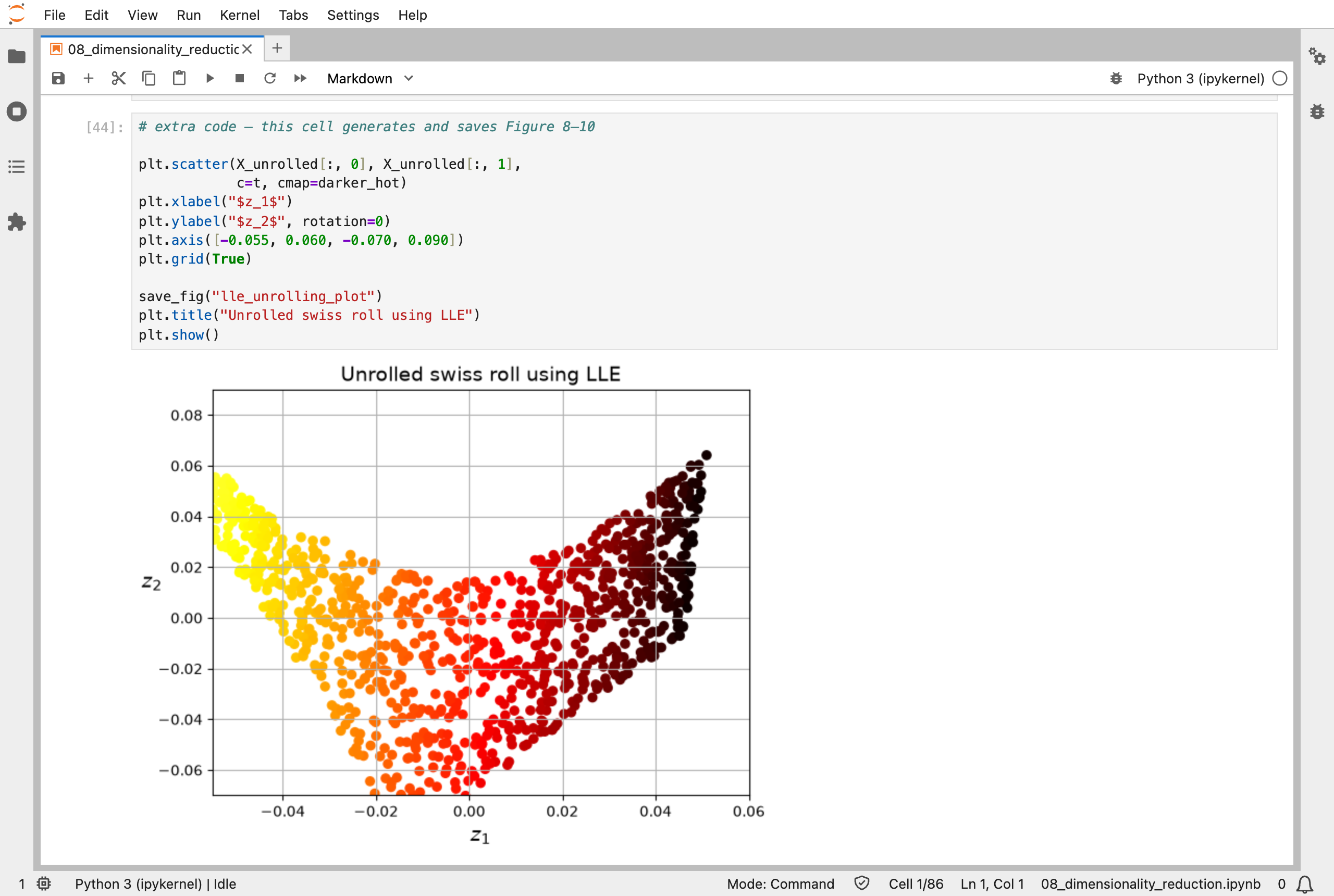
LLE unrolled the Swiss roll: the colours now run smoothly from one end to the other
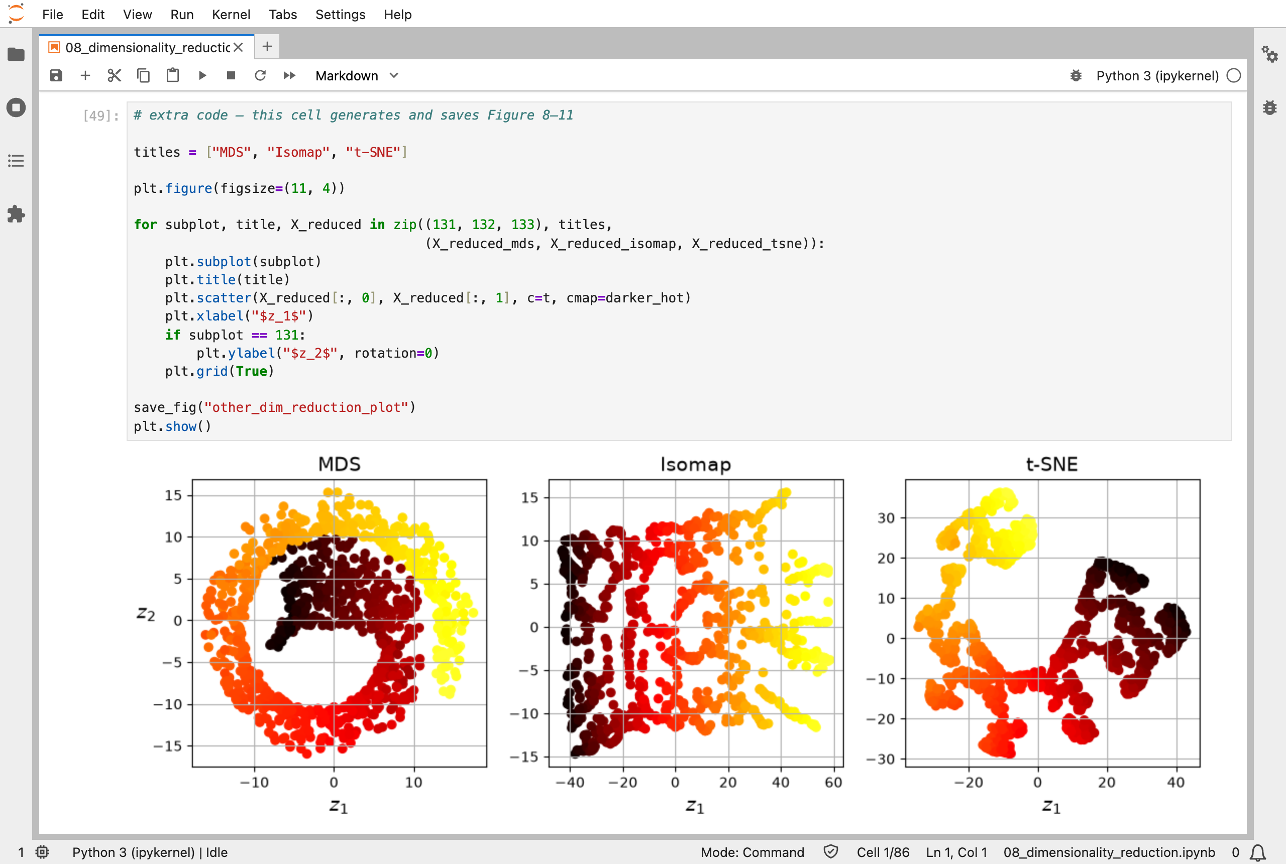
Three other methods laying the Swiss roll out in 2D: MDS (multidimensional scaling), Isomap (isometric mapping), and t-SNE, which keeps neighbours together but breaks the roll into pieces
Next, Scikit-Learn (Part 9) works through chapter 9: unsupervised learning, finding groups in data with no labels at all.