The problem in this project is made up, and I will say so now. The book invents a company that wants to estimate what a typical house costs in each California district, so that an investor can decide where to buy. No one needs these estimates, because the data already holds the real price for every one of its 20,640 districts: it comes from the 1990 census, one row for each district, with facts such as its location, the age of its houses, its rooms, its population, and its incomes, and the median price of a house there.
The book uses it because the answers are known, so that I can check my work. I hide some districts from the model, let it learn the link between facts and price from the rest, and then ask it to guess the prices of the hidden ones and compare its guesses with the truth. That is the same job that real valuation tools do for homes, where the price is not known and the facts are. What matters in this chapter is the sequence of steps for a project of this kind, which carry over to real problems, and not the prices, which are 1990 prices in any case. I explain why below.
The error for one district is the gap, in dollars, between the model's guess and the real price. To score the whole model, I average the errors over districts that it has never seen. On 4,128 such districts, the average error of the final model was about $26,000. Half of the districts had an error under about $15,500, which is about 9% of the price, and the worst errors were about $300,000. The typical district's price is $180,000.
In Part 1, I ran the small example from the first chapter of the Hands-On Machine Learning book. The second chapter is a whole project, from raw data to a tested model.
Key Points
The eight steps of a machine learning project:
- Look at the big picture: decide what the prediction will be used for, and how to score it (here, by the size of its errors in dollars, averaged over many districts)
- Get the data: 20,640 California districts, with 10 columns each
- Explore the data: histograms, a map, and correlations
- Prepare the data: fill in missing values, encode text, scale the numbers, all in one pipeline
- Select and train a model: a linear model (a straight line through the data), a decision tree (a flowchart of yes-or-no questions about a house, such as "is the median income above 5?", that ends in a price), then a random forest (many decision trees, whose prices are averaged)
- Fine-tune the model: try different settings for the model and the data preparation, and keep the ones that score best, either by trying every combination from a short list (grid search) or by trying random combinations (randomized search)
- Present the solution
- Launch, monitor, and maintain the system
What I learned from it:
- The test set is set aside first, before looking at the data, so that it cannot influence any decision.
- A pipeline keeps every preparation step together, so the same steps run on the training data, the test data, and any new data.
- A model can look perfect on the houses it learned from and still be poor on new ones. The decision tree got the price of every training house exactly right, an error of $0, because it had memorised them. On houses it had not seen, its typical error was about $67,000.
Quick Example
A model's score on the districts it learned from tells me almost nothing, because it can simply remember them. To find out how good it really is, I have to score it on districts it has not seen. I have 16,512 training districts, and the test set is off limits until the end, so the code below makes its own held-back districts out of the training ones, like this:
- Cut the 16,512 districts into 10 equal groups of about 1,650.
- Train the model on 9 of the groups, about 14,860 districts.
- Score it on the 1 group that it did not train on. That is its validation: a check on districts it has not seen.
- Do steps 2 and 3 again, holding back a different group each time, until every group has been held back once. That is 10 rounds, and 10 scores.
- Average the 10 scores.
Every district gets a turn as a held-back district, and no district is ever scored by a model that trained on it. The name for all this is 10-fold cross-validation. "Validation" is the check on held-back districts, "cross" means that the groups swap roles, and each of the 10 groups is a "fold", like a fold of a sheet of paper. The model here is a random forest, many decision trees whose answers are averaged. A decision tree is a flowchart of yes-or-no questions about a house, and Part 6 shows how one is grown.
The model is bundled with the steps that prepare the data, such as filling in missing values and scaling the numbers, into a single object called a pipeline. That matters in the ten rounds: each round prepares its data using only the 9 parts it trains on, so nothing from the part left out leaks into the preparation:
PYTHON
1from sklearn.ensemble import RandomForestRegressor
2from sklearn.model_selection import cross_val_score
3from sklearn.pipeline import make_pipeline
4
5forest_reg = make_pipeline(preprocessing,
6                           RandomForestRegressor(random_state=42))
7forest_rmses = -cross_val_score(forest_reg, housing, housing_labels,
8                                scoring="neg_root_mean_squared_error", cv=10)
Here is how each model did when I ran the notebook. Each score below summarises the errors over many districts into one number in US dollars, where lower is better. It is called the RMSE, and it is larger than the plain average error. I explain how it is worked out, and why, in the questions below:
| Model | How it was measured | RMSE |
|---|---|---|
| Linear regression | on the houses it trained on | 68,648 |
| Decision tree | on the houses it trained on | 0 |
| Decision tree | on held-back districts (10 rounds, called 10-fold cross-validation) | 67,153 |
| Random forest | on held-back districts (10 rounds, called 10-fold cross-validation) | 47,003 |
| Random forest, grid search | on held-back districts (3 rounds, called 3-fold cross-validation), best | 43,954 |
| Random forest, randomized search | on held-back districts (3 rounds, called 3-fold cross-validation), best | 41,983 |
| The final model | on the test set | 41,536 |
The test set is 20% of the districts, 4,128 of the 20,640, set aside at the start. The other 16,512 are the training districts, and each cross-validation score covers all of them: every one is held back once, in one of the rounds, and scored by a model that did not learn from it. So the cross-validation scores are each worked out over 16,512 districts, and the last one over the 4,128 test districts.
What the two searches did. A model has settings that I choose before training starts, such as how many questions each tree may consider at once. These are called hyperparameters, and the best values are not known in advance. Two settings are searched here: n_clusters, how many geographic groups the pipeline sorts the districts into by latitude and longitude, and max_features, how many of the columns each tree may look at when it chooses a question.
- Grid search tries every combination from a short list that I write down. The notebook's list is 3 values of
n_clusterswith 3 ofmax_features, plus 2 with 3 more: 15 combinations. Each combination is scored with 3-fold cross-validation, and the best one wins. It is thorough, and the work grows quickly as the lists get longer. - Randomized search is given a range for each setting, such as any whole number from 3 to 49 for
n_clusters, and picks random combinations from it, here 10. It covers a wider range with the same amount of work, and is usually better when there are many settings or I do not know where the good values are.
Both ended with a better score than the random forest's 47,003 with its default settings: 43,954 from the grid, and 41,983 from the random search.
What training means here
Every .fit() call trains a model, and this project trains about 110 of them, which is why it takes minutes rather than seconds:
| What | Models trained |
|---|---|
| Linear regression and a decision tree, once each | 2 |
| 10-fold cross-validation of the tree, the linear model and the random forest | 30 |
| One more random forest, on the whole training set | 1 |
| Grid search: 15 combinations × 3 folds, plus a final refit | 46 |
| Randomized search: 10 combinations × 3 folds, plus a final refit | 31 |
88 of those are random forests, each made of 100 decision trees, so the project grows about 8,800 trees in all. None of them trains the way a neural network does:
- Linear regression is worked out directly, in one calculation (least squares).
- A decision tree grows one split at a time, each time choosing the question that best divides the districts, until every leaf holds districts with the same value. That is why it scored exactly 0 on its own training data. Part 6 is a whole chapter on decision trees.
- A random forest grows 100 trees, each on a random sample of the districts, and averages their answers. One tree memorises its training data and changes a lot with small changes to the data, but 100 different trees make different mistakes, and averaging cancels many of them out. Part 7 covers random forests, and other ways of combining trees.
My MiniGPT model starts from 826,433 random numbers and nudges every one of them thousands of times, using backpropagation to find which way each should move. Nothing here is nudged: every model is either worked out exactly or grown one decision at a time. Scikit-Learn does have models that train by nudging, such as SGDRegressor, and small neural networks trained with backpropagation, such as MLPRegressor, but this project does not use them.
Which facts matter most?
The notebook answers this two ways, and I added a third check of my own. They disagree, which is the lesson.
- Correlation: a score from −1 to 1 for how closely a column moves with the price. Median income is far ahead at 0.69. The next best, rooms per house, is 0.14.
- The forest's own ranking: after training, the random forest reports how much each column helped. Median income is first, at 0.19, then being inland, at 0.08.
- Leaving columns out (my own check, not in the book): I trained a forest on the plain numeric columns, scored on houses held back from training (3-fold cross-validation), and then removed one column at a time:
| Columns used | Typical error ($) |
|---|---|
| All the numeric columns | 50,416 |
| Without longitude | 63,210 |
| Without latitude | 62,235 |
| Without median income | 51,883 |
| Without the age of the houses | 48,786 |
| Latitude and longitude only | 53,762 |
| Median income only | 96,134 |
Income is the strongest single link, but removing it barely hurts, because other columns carry the same information: richer districts are also in particular places. Removing location hurts most, and location alone does nearly as well as everything together. Removing the age of the houses made the error slightly smaller, which tells me that column is mostly noise. It is one run, so I would not read much into differences of a thousand dollars.
So "how closely related" depends on how I ask. Columns that overlap share the credit, and a high score shows that two things move together, not that one causes the other.
Why a forest, and what else could I have used?
The authors did not pick a forest in advance. They tried a linear model, a decision tree and a random forest, scored all three on houses held back from training, and kept the best, which was the forest. For a table of facts about districts, that is a sensible choice. These are the main options, with their strengths and weaknesses. This is my own summary, and the later parts show the evidence for each.
| Model | Strength | Weakness |
|---|---|---|
| Linear regression (Part 4), from the 1800s | Simple, fast, easy to explain: one number per column | Cannot bend to fit curves, and gives unreliable numbers when columns overlap (mine gave the island category a coefficient of 196,583 on very few houses) |
| Decision tree (Part 6), 1980s | Easy to read as a flowchart | Memorises its training data: an error of $0 on the training houses and $67,153 on new ones |
| Random forest (Part 7), 2001 | Strong on tables with little tuning, and much less prone than one tree to memorising the training data (the forest's error was 47,003 on new houses, against the tree's 67,153) | Slower, and no longer a flowchart that a person can read |
| Gradient-boosted trees (Part 7), 2000s | Often the most accurate on tables today | More settings to tune, and easier to overfit |
| Neural networks (Part 10 onward), modern | The best for images, sound and text | Need much more data and tuning, and are often no better than trees on a table like this |
Random forests are not new, but they are still a standard first choice for tables of data. Neural networks are what has changed in the last decade. They have taken over images and language, but trees have mostly kept the tables.
Running the notebook in Jupyter
The project is in the chapter 2 notebook that goes with the book, 02_end_to_end_machine_learning_project.ipynb. I ran the project part of it, everything up to the test set, and then looked through the results in JupyterLab. The whole run took about 6 minutes on my Mac Studio, most of it in the two searches.
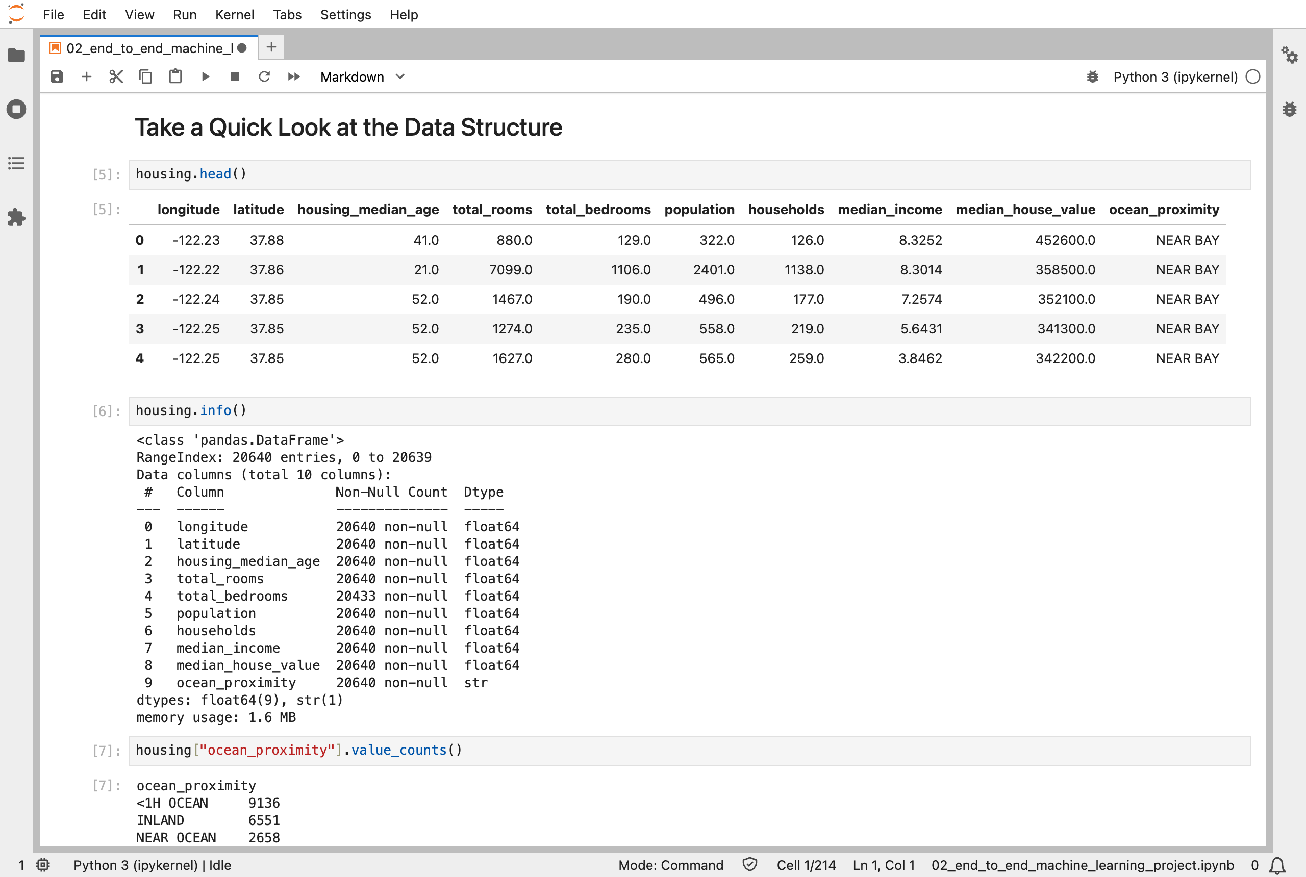
I loaded the data: 20,640 districts, one row each, with the median house value in the ninth column
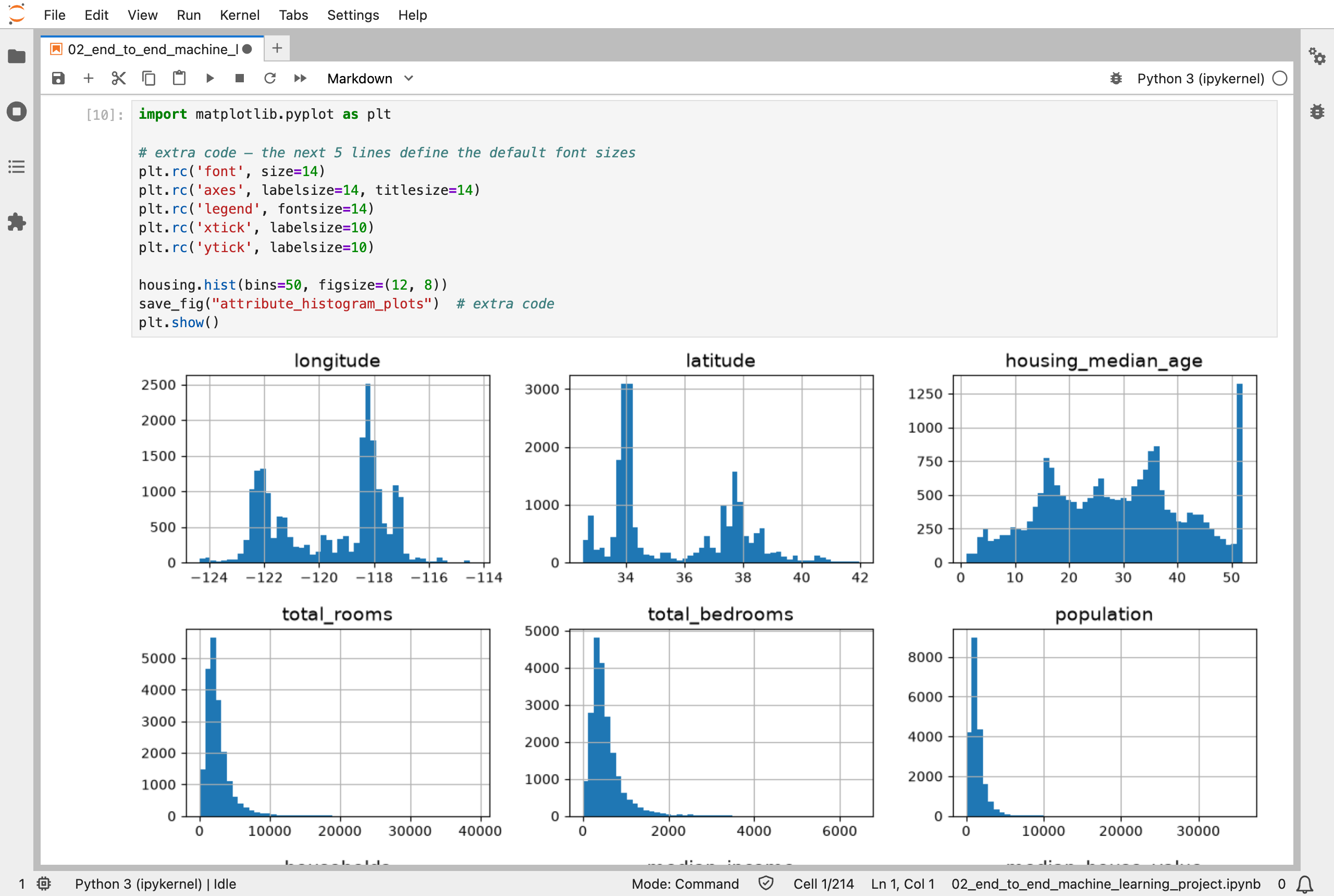
I plotted a histogram of every column: housing_median_age is capped at 52, which shows as a tall spike on the right
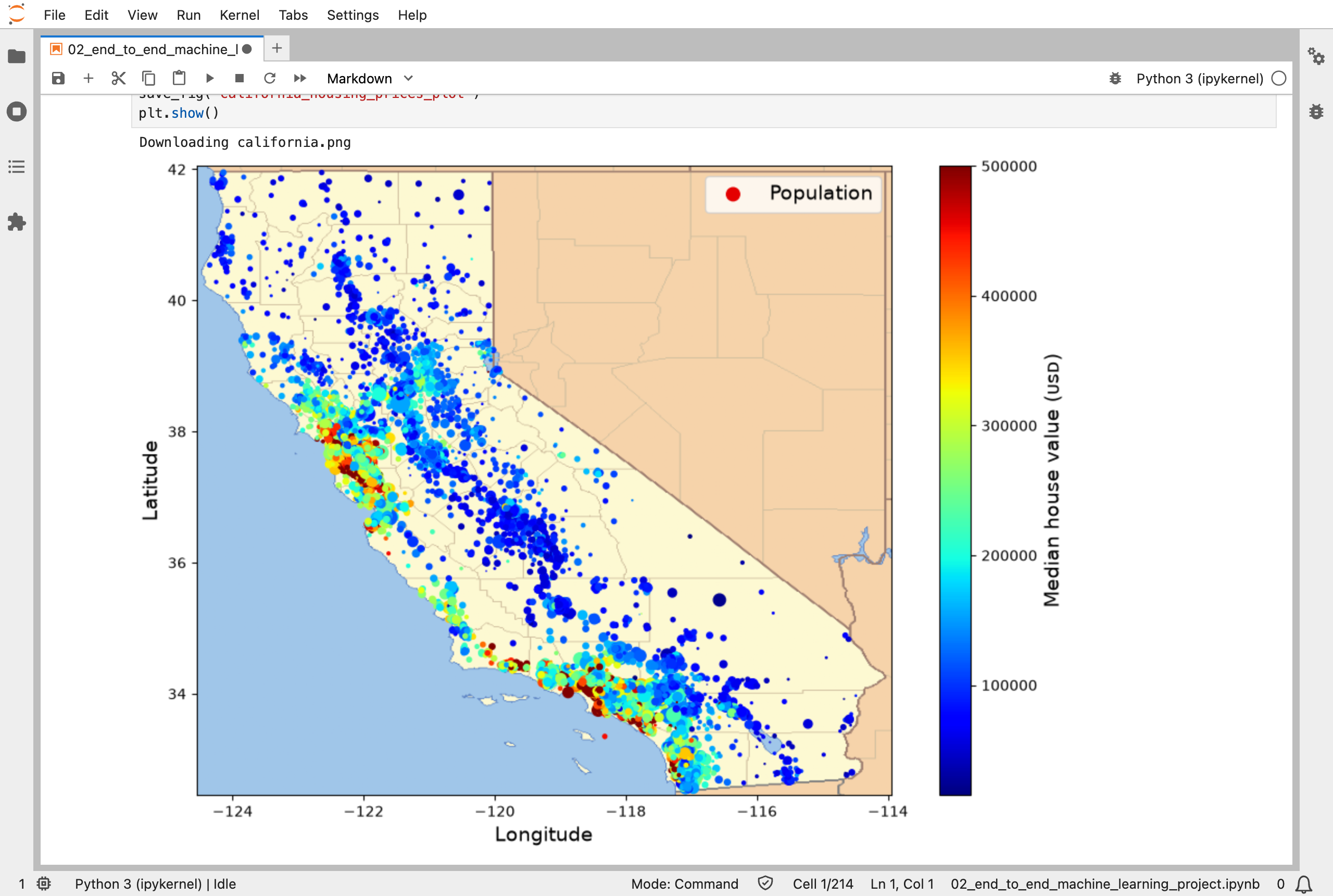
I put the districts on a map of California: the most expensive, in red, are along the coast, around the Bay Area and Los Angeles
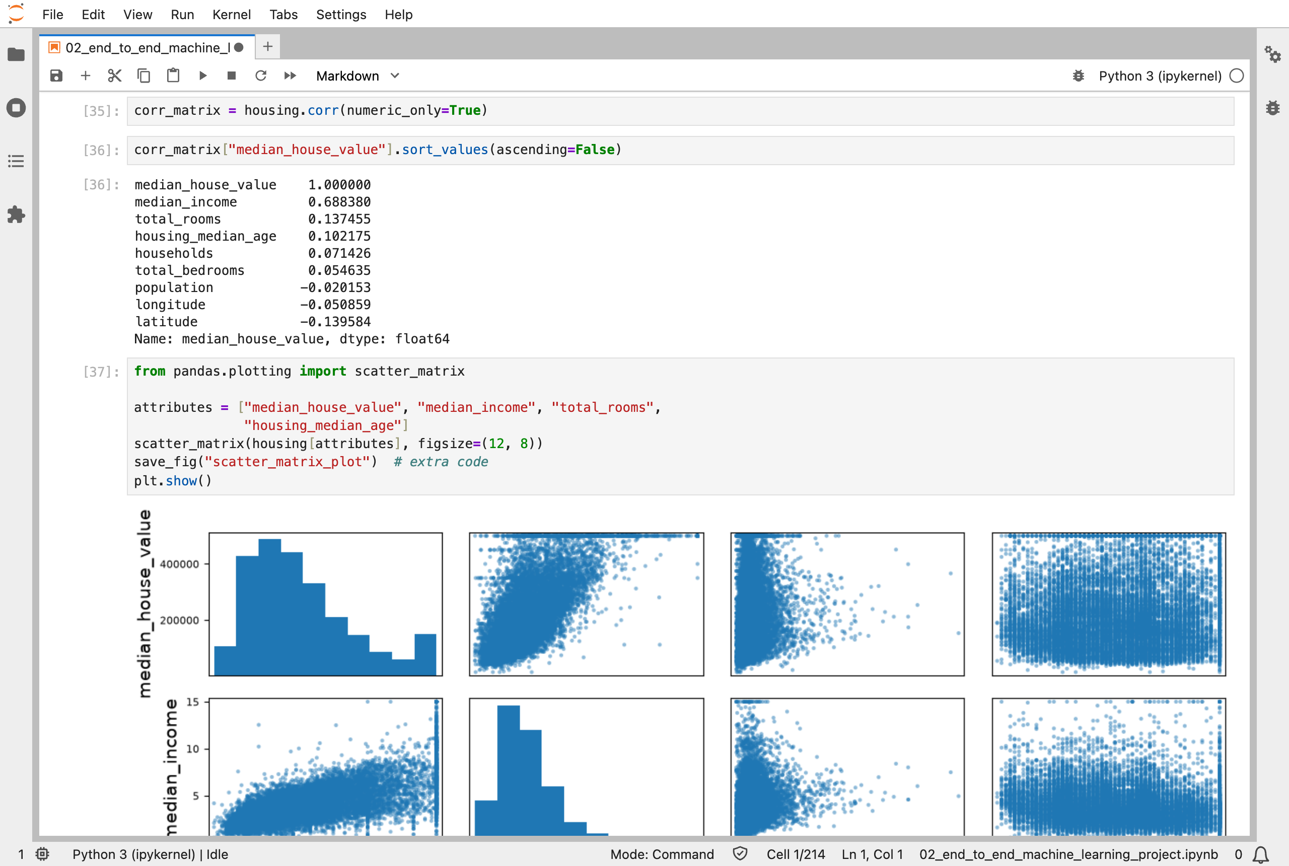
I looked for correlations: median_income is the column most closely related to house value, at 0.69
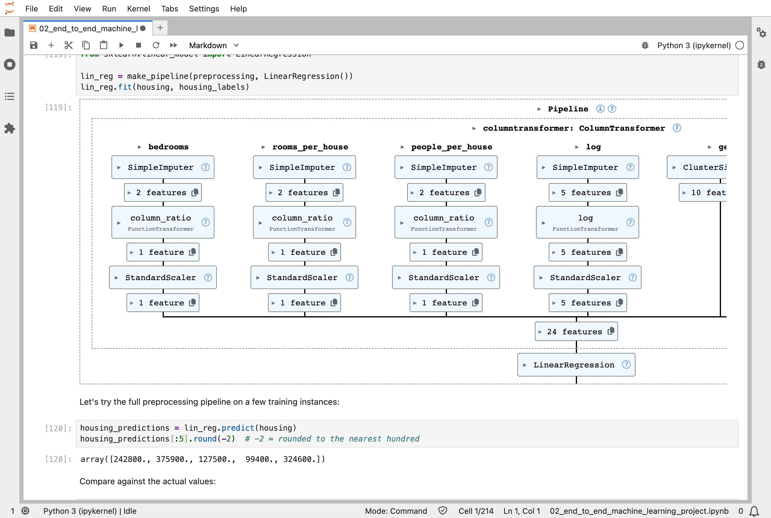
Scikit-Learn drew the preprocessing pipeline that feeds the linear regression: each kind of column gets its own steps, and 24 features come out
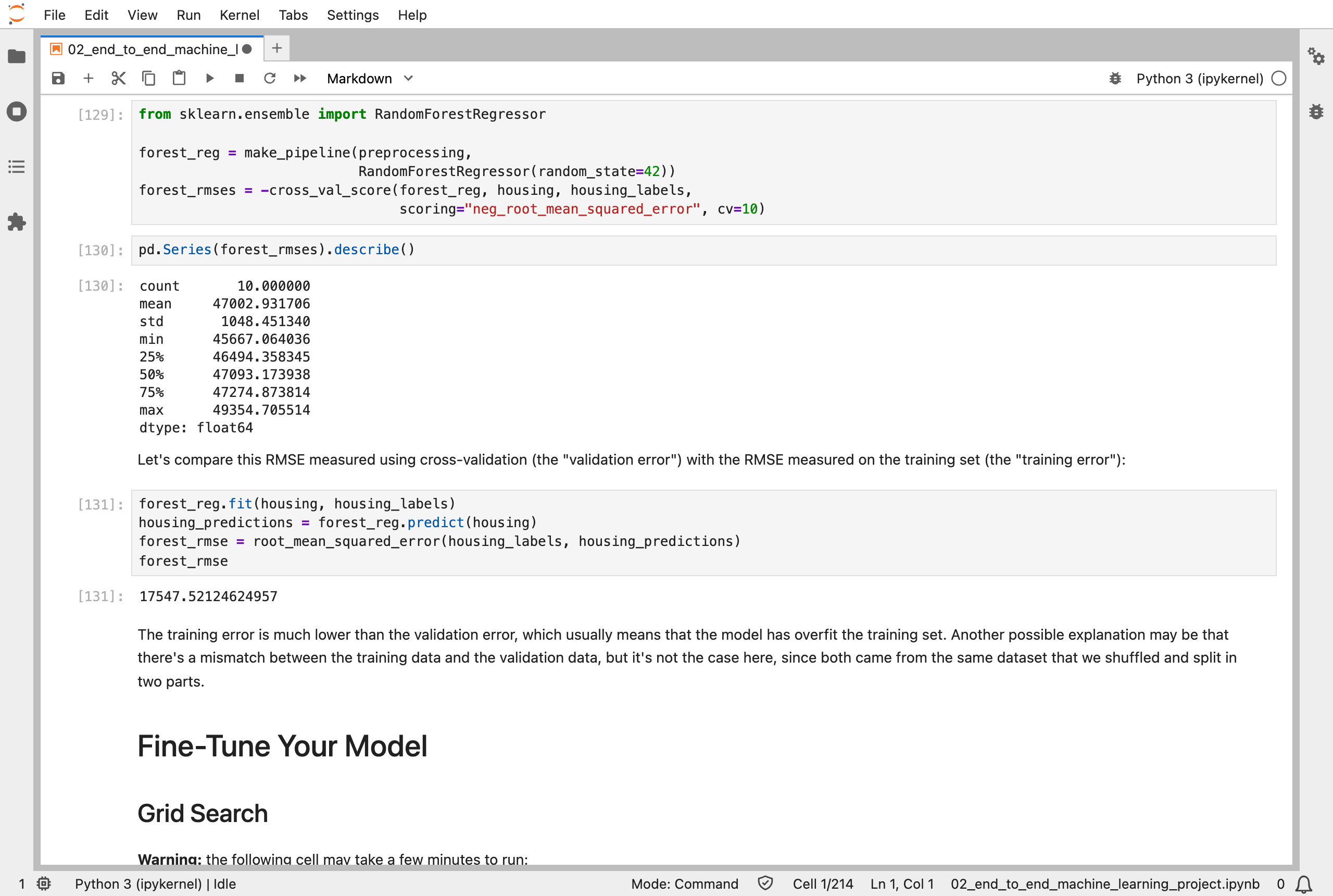
A random forest was wrong by about 47,000 on houses held back from training, but only 17,548 on the houses it trained on, so it is still overfitting: it does much better on what it has seen
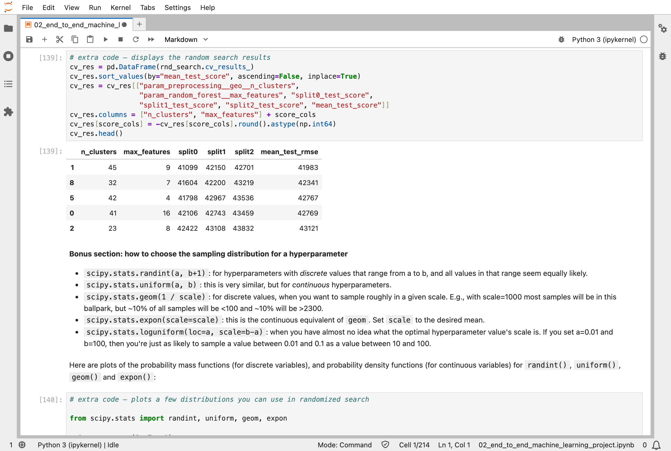
Randomized search tried different numbers of geographic clusters and features: the best combination scored 41,983
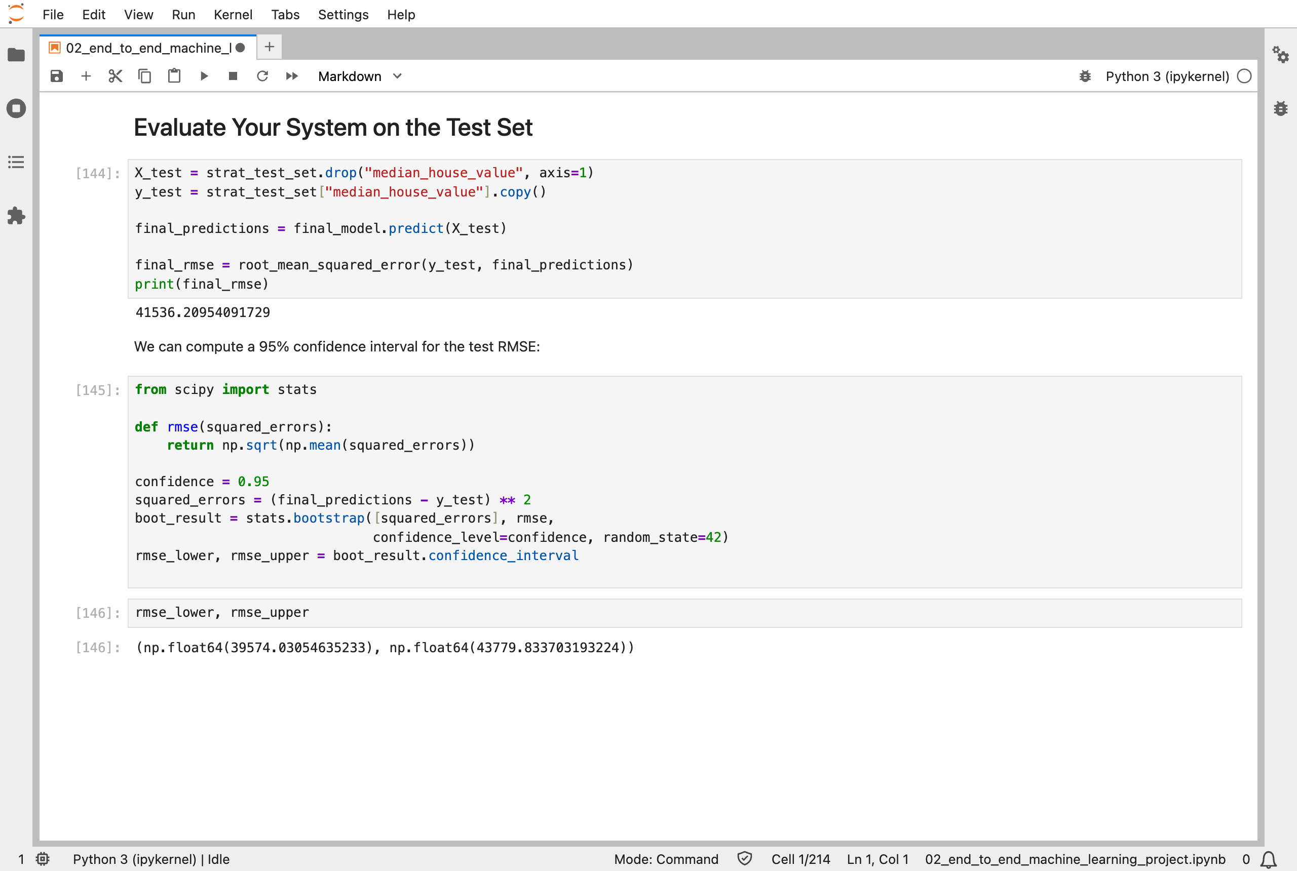
Finally, I tested the model on the test set, which it had never seen: an RMSE of 41,536, with a 95% confidence interval from 39,574 to 43,780
Next, Scikit-Learn (Part 3) works through chapter 3: classification, with handwritten digits.