Scikit-Learn (Part 5)

Neil Haddley • October 12, 2026

Support vector machines: the widest street between two classes, kernels for curved boundaries, and an SVM trained both directly and by gradient descent

AI Pythonmachine-learningscikit-learnsupport-vector-machineskernelsirismoons

In Part 4, I fitted lines to points. This chapter of the Hands-On Machine Learning book draws a line between two groups instead. The task is a classic one: decide, from the petal length and width, whether an iris flower is an Iris virginica or one of the other two species. The data is real, 150 flowers measured in the 1930s, and small enough that I can picture it as dots on a page. Using it for a real purpose is not the point. It is a clear place to learn a method that is used on bigger data.

Many lines would separate the two groups of flowers. The method in this chapter, the support vector machine (SVM), picks the line with the widest empty strip on either side of it, which the book calls a street. In my run, a flower with petals 5.5 cm long and 1.7 cm wide came out as an Iris virginica, and one with petals 5.0 cm by 1.5 cm did not.

Key Points

The lesson: a good boundary is one that sits as far as possible from both groups, because that leaves room for new flowers that are a little different. Only the flowers on the edge of the street decide where it goes, and they are the support vectors. The rest could move around without changing anything. That also means the street's width depends on the units: if one measurement is in much bigger numbers than another, it dominates, so the measurements are rescaled first.

What I learned from it:

An SVM ignores most of its training data. Only the flowers on the edge of the street matter.
A setting called C decides the trade-off between a wide street and a few flowers on the wrong side of it. Small C, a wide and forgiving street; large C, a narrow street that gets more of the training flowers right.
A kernel lets an SVM draw a curved boundary without computing any extra curved features, using a shortcut that compares pairs of flowers directly. A second setting, gamma, says how far each flower's influence reaches, and so how wiggly the curve is.

The chapter also turns the idea around for predicting numbers, which I do not go into here.

Quick Example

A linear SVM that decides whether an iris is an Iris virginica, from its petal length and width:

PYTHON

1import numpy as np
2from sklearn.datasets import load_iris
3from sklearn.pipeline import make_pipeline
4from sklearn.preprocessing import StandardScaler
5from sklearn.svm import LinearSVC
6
7iris = load_iris(as_frame=True)
8X = iris.data[["petal length (cm)", "petal width (cm)"]].values
9y = (iris.target == 2)  # Iris virginica
10
11svm_clf = make_pipeline(StandardScaler(),
12                        LinearSVC(C=1, dual=True, random_state=42))
13svm_clf.fit(X, y)

When I ran it, a flower with petals 5.5 cm long and 1.7 cm wide came out as an Iris virginica, and one with petals 5.0 cm by 1.5 cm did not. Their scores, positive on the Iris virginica side of the boundary and negative on the other, were 0.66 and −0.22.

The chapter's extra material trains the same kind of model in two ways, on the same flowers, and compares them:

How it was trained	Intercept	Petal length weight	Petal width weight
Scikit-Learn's `SVC`, solved directly	−15.517	2.271	2.713
The notebook's `MyLinearSVC`: random start, 60,000 steps of gradient descent	−15.568	2.281	2.716

What training means here

Scikit-Learn's SVC (support vector classifier) does not nudge. Finding the widest street is a well-understood mathematical problem, and SVC hands it to a specialised solver, LIBSVM (a library for SVMs), which works on it two numbers at a time, solving each small piece exactly, rather than taking small steps along a slope.

The chapter's extra material then trains the same model by gradient descent, exactly like Part 4: start from random weights, work out which way the error slopes, step downhill, and repeat, 60,000 times. It lands within about 0.05 of the direct answer. So an SVM can be trained either way, like the straight line in Part 4.

My MiniGPT model can only be trained the nudging way: no one knows a direct calculation that finds its 826,433 numbers.

There are no Dumb Questions

Q: What is the kernel trick?

A: A way to get a curved boundary without adding curved features. The SVM's calculation only needs to compare pairs of instances, and a kernel does that comparison as if the extra features were there, without ever computing them.

Q: Why did gradient descent not land exactly on SVC's answer?

A: 60,000 steps brought it within about 0.05 of the direct answer: close, but each small step only approaches the bottom of the valley, and the notebook stops after 60,000 of them.

Q: What do C and gamma do?

A: Both trade smoothness against fit. A small C allows a wider street with a few flowers inside it; a large C narrows the street to get more flowers right. A larger gamma makes each training flower's influence reach less far, so the boundary wiggles around individual flowers.

Q: Are support vector machines still used?

A: Less than when the book was written, and I would not reach for one first. They work well on small or medium datasets with many features, but training gets slow as the number of examples grows, and for tables of data gradient-boosted trees (see Part 7) are usually more accurate. Kernels are now rare outside small problems. The idea of the widest street is still a good way to think about what a boundary should do.

Running the notebook in Jupyter

The chapter is in the notebook that goes with the book, 05_support_vector_machines.ipynb. I ran everything before the exercise solutions, which took about 10 seconds on my Mac Studio, and then looked through the results in JupyterLab.

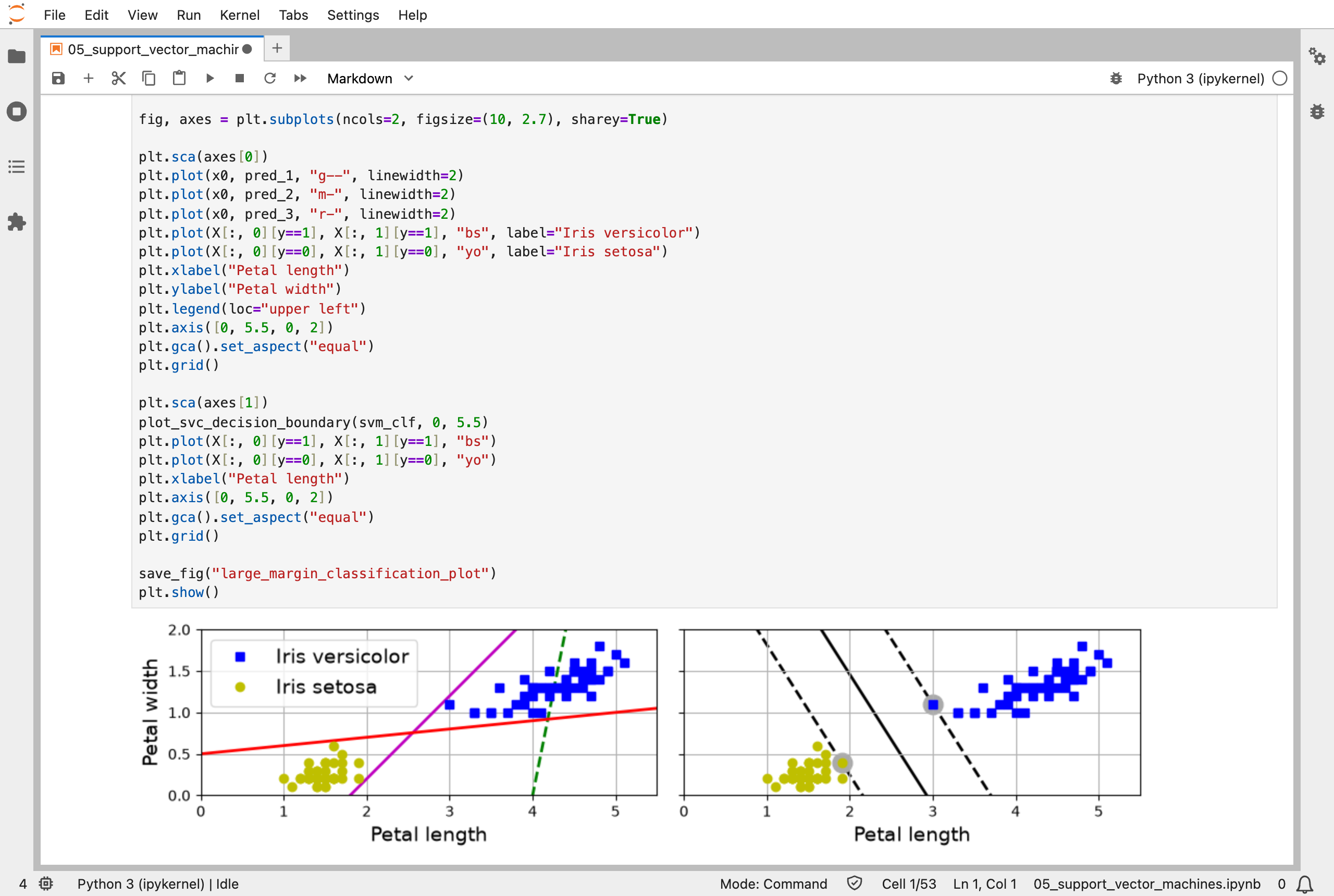
On the left, three lines that separate the flowers badly or barely; on the right, the SVM's widest street, with its support vectors circled

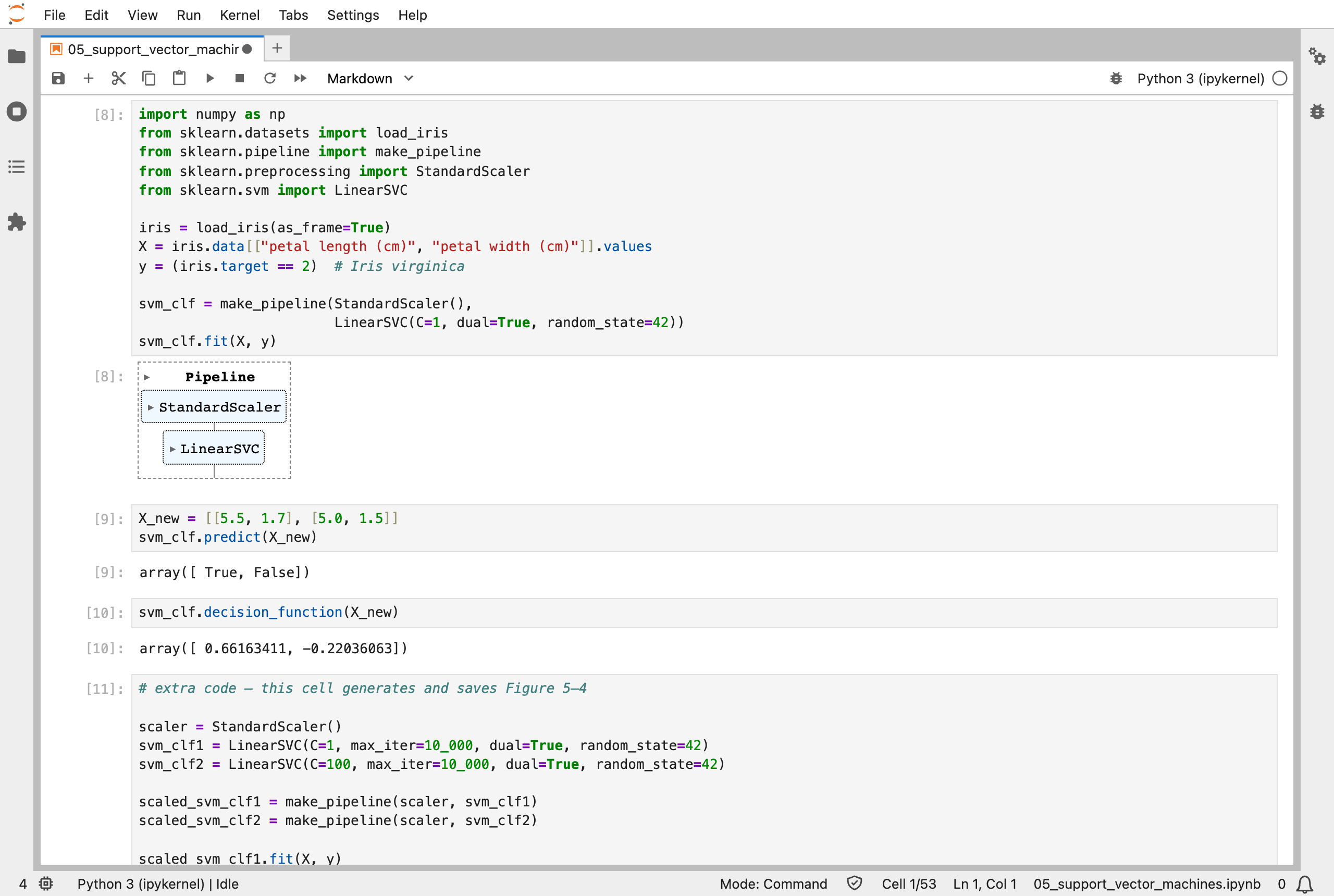
I trained a linear SVM to spot Iris virginica, and it classified two new flowers: one yes, one no

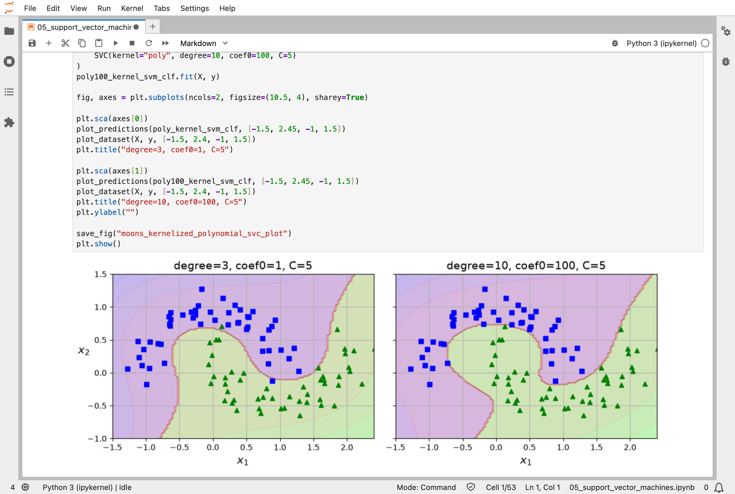
A polynomial kernel lets the SVM curve its boundary around the two moons

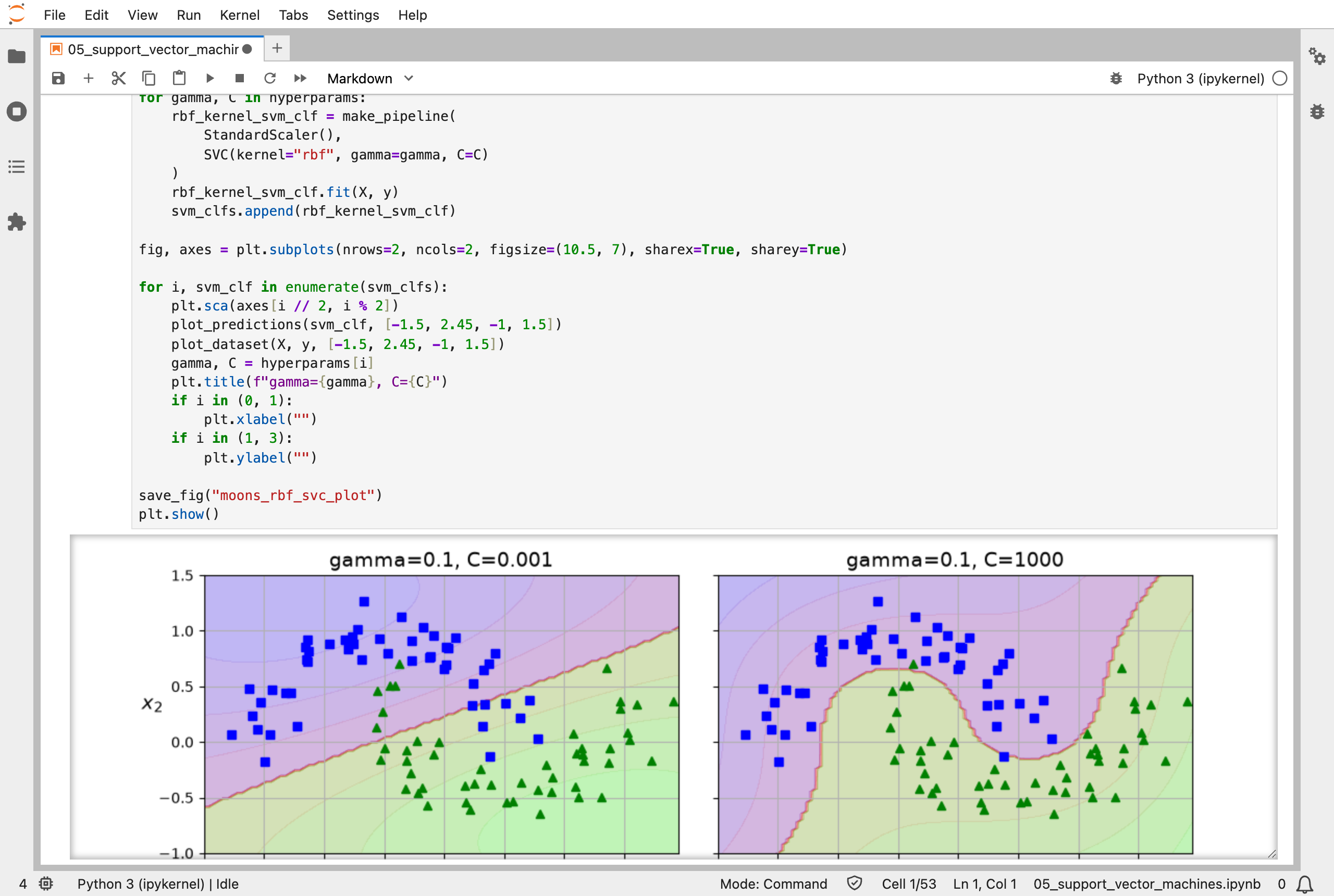
The Gaussian RBF kernel with different settings: a small C gives a smooth boundary, and a large C follows the training data closely

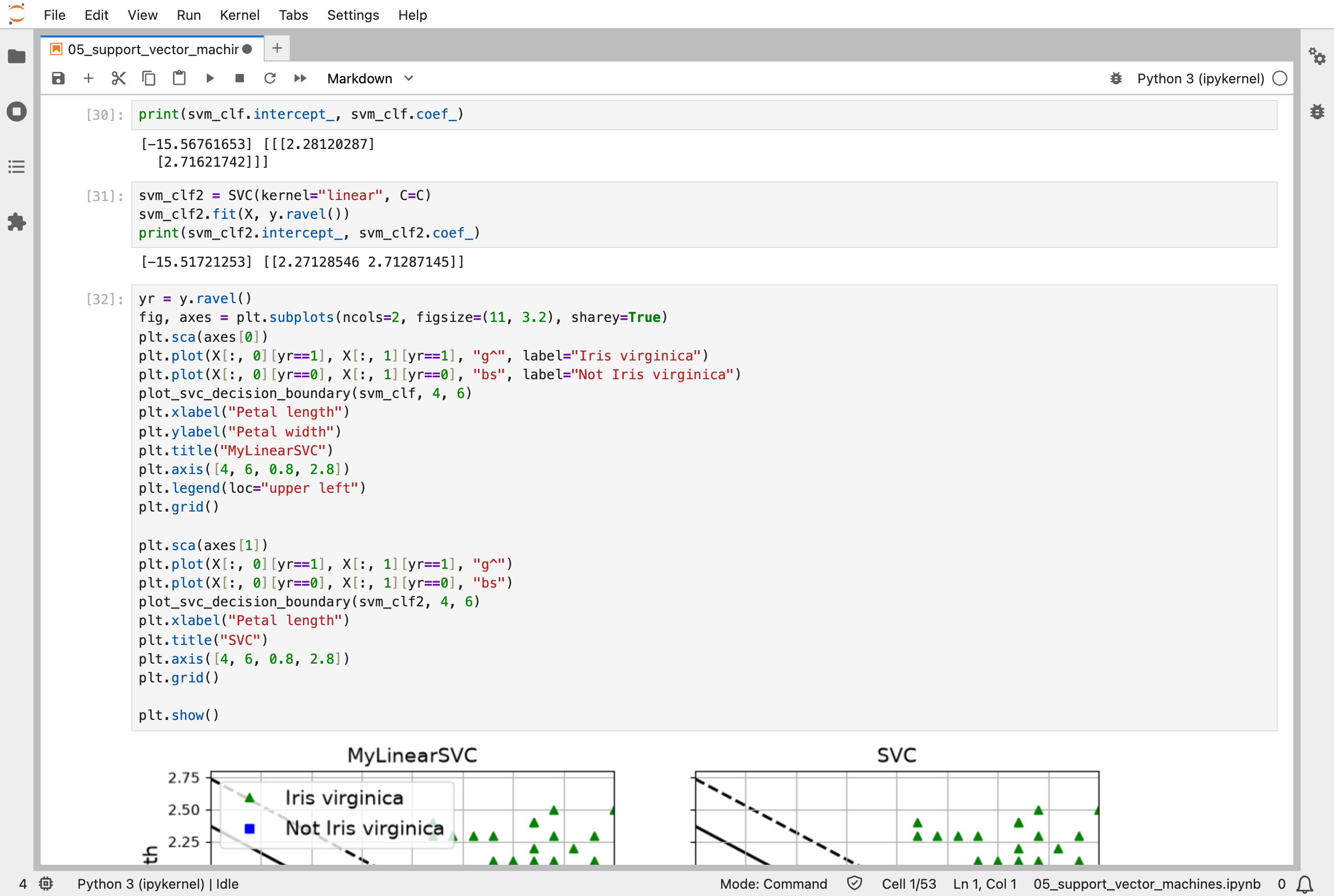
The same SVM trained by gradient descent and by Scikit-Learn's SVC: the two answers agree to within about 0.05

Next, Scikit-Learn (Part 6) works through chapter 6: decision trees.

Scikit-Learn (Part 4)

Training linear models: the same line worked out directly and found by gradient descent, then curves, regularization, and logistic regression

Next in series →

Scikit-Learn (Part 6)

Decision trees: a model that asks one question at a time, grown split by split, and why it needs holding back